<?xml version="1.0" encoding="utf-8"?><feed xmlns="http://www.w3.org/2005/Atom" xml:lang="en"><generator uri="https://jekyllrb.com/" version="4.4.1">Jekyll</generator><link href="https://intsystems.github.io/feed/blog.xml" rel="self" type="application/atom+xml" /><link href="https://intsystems.github.io/" rel="alternate" type="text/html" hreflang="en" /><updated>2026-08-26T11:43:04+00:00</updated><id>https://intsystems.github.io/feed/blog.xml</id><title type="html">Intelligent Systems | Blogs</title><subtitle>Intelligent Systems Department at MIPT — news, courses, people and research</subtitle><entry xml:lang="en"><title type="html">Multiobjective Tree-Structured Parzen Estimator (MOTPE): Bayesian Optimization for the Real World</title><link href="https://intsystems.github.io/materials/blog/motpe/" rel="alternate" type="text/html" title="Multiobjective Tree-Structured Parzen Estimator (MOTPE): Bayesian Optimization for the Real World" /><published>2026-05-21T00:00:00+00:00</published><updated>2026-05-21T00:00:00+00:00</updated><id>https://intsystems.github.io/materials/blog/motpe</id><content type="html" xml:base="https://intsystems.github.io/materials/blog/motpe/"><![CDATA[<h2 id="multiobjective-tree-structured-parzen-estimator-motpe-bayesian-optimization-for-the-real-world">Multiobjective Tree-Structured Parzen Estimator (MOTPE): Bayesian Optimization for the Real World</h2>

<h2 id="introduction-the-problem-with-real-world-problems">Introduction: The Problem with Real-World Problems</h2>

<p>Many of us are familiar with optimizing a single metric, like minimizing the error rate of a machine learning model. However, real-world problems are rarely that simple. They often involve juggling multiple, <strong>conflicting objectives</strong> simultaneously.</p>

<p><strong>Real-world examples:</strong></p>

<ul>
  <li><strong>Neural Network Design:</strong> High accuracy <em>vs.</em> low inference time (faster predictions).</li>
  <li><strong>Mechanical Engineering:</strong> Maximum power <em>vs.</em> minimum fuel consumption.</li>
  <li><strong>Cloud Computing:</strong> Low cost <em>vs.</em> high performance.</li>
</ul>

<p>These objective functions are often:</p>
<ul>
  <li><strong>Expensive to evaluate</strong> (each evaluation takes hours or days).</li>
  <li><strong>Black-box</strong> (no simple mathematical formula).</li>
  <li>Defined on <strong>complex search spaces</strong> (mixed real, integer, categorical, and conditional parameters like “if layer X exists, then set parameter Y”).</li>
</ul>

<p>So, what algorithm can handle all of this efficiently?</p>

<h2 id="the-limitations-of-existing-methods">The Limitations of Existing Methods</h2>

<p>The standard tool for expensive black-box optimization is <strong>Bayesian Optimization (BO)</strong> using <strong>Gaussian Processes (GPs)</strong>.</p>

<p><strong>GP-based methods</strong> (like PESMO, ParEGO, SMS-EGO) are powerful, but they have major drawbacks:</p>
<ul>
  <li>❌ Not suitable for non-continuous or conditional (tree-structured) spaces.</li>
  <li>❌ High computational complexity: <strong>O(n³)</strong> — they scale poorly with the number of observations.</li>
  <li>❌ Approximation tricks help but cause performance degradation.</li>
</ul>

<p><strong>Single-Objective TPE</strong> (Tree-Structured Parzen Estimator) is a great alternative that:</p>
<ul>
  <li>✅ Naturally handles complex, conditional spaces.</li>
  <li>✅ Scales to ~1000 observations and tens of variables.</li>
  <li>✅ Outperforms GP-based methods on single-objective HPO.</li>
  <li>❌ <strong>But:</strong> It is designed for single-objective only!</li>
</ul>

<h2 id="enter-motpe-multiobjective-tree-structured-parzen-estimator">Enter MOTPE: Multiobjective Tree-Structured Parzen Estimator</h2>

<p><strong>MOTPE</strong> (Ozaki et al., 2020/2022) extends the powerful TPE algorithm to handle <strong>multiple objectives</strong>. It is designed to be:</p>

<table>
  <thead>
    <tr>
      <th style="text-align: left">Property</th>
      <th style="text-align: left">How MOTPE Achieves It</th>
    </tr>
  </thead>
  <tbody>
    <tr>
      <td style="text-align: left"><strong>Handles complex spaces</strong></td>
      <td style="text-align: left">Uses Parzen estimators (density estimation) per parameter, not a global GP.</td>
    </tr>
    <tr>
      <td style="text-align: left"><strong>Scalable</strong></td>
      <td style="text-align: left">O(k log k) per iteration vs. O(n³) for GP methods.</td>
    </tr>
    <tr>
      <td style="text-align: left"><strong>Parallelizable</strong></td>
      <td style="text-align: left">Asynchronous parallelization without wait time.</td>
    </tr>
    <tr>
      <td style="text-align: left"><strong>Limited budget</strong></td>
      <td style="text-align: left">Efficiently approximates the Pareto front with few evaluations.</td>
    </tr>
  </tbody>
</table>

<h2 id="how-it-works-the-core-idea">How It Works: The Core Idea</h2>

<h3 id="1-the-split-rule">1. The Split Rule</h3>

<p>In single-objective TPE, observations are split into “good” (below a quantile threshold y*) and “bad” (above). For multiple objectives, MOTPE uses a dominance-based split:</p>

<ul>
  <li><strong>Good set (l(xᵢ)):</strong> Points that are <strong>either</strong> dominated by <strong>or</strong> incomparable to the current Pareto front approximation Y*.</li>
  <li><strong>Bad set (g(xᵢ)):</strong> Points that weakly dominate Y* (i.e., are clearly worse).</li>
</ul>

<p>This allows the algorithm to learn which parameter values tend to produce good (non-dominated or diverse) solutions.</p>

<h3 id="2-greedy-splitting-with-hypervolume">2. Greedy Splitting with Hypervolume</h3>

<p>To select the top γ% of observations for the good set, MOTPE:</p>
<ol>
  <li>Sorts observations by nondomination rank (Pareto sorting).</li>
  <li>Greedily adds full fronts.</li>
  <li>For the remaining slots, solves the <strong>Hypervolume Subset Selection Problem (HSSP)</strong> using a greedy algorithm with a (1 — 1/e)-optimality guarantee.</li>
</ol>

<p>Points in the good set are then <strong>weighted by their hypervolume contribution</strong> — points that improve the Pareto front more get higher weight in the density model.</p>

<h3 id="3-the-acquisition-function-expected-hypervolume-improvement-ehvi">3. The Acquisition Function: Expected Hypervolume Improvement (EHVI)</h3>

<p>MOTPE uses <strong>Expected Hypervolume Improvement (EHVI)</strong> as its acquisition function. Remarkably, after derivation, EHVI simplifies to:</p>

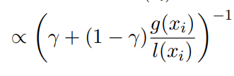
<p><img src="/images/blog/EHVI.png" alt="alt text" /></p>

<p>This means: <strong>To maximize EHVI, simply maximize the ratio l(xᵢ) / g(xᵢ)</strong> — exactly the same as in single-objective TPE! No complex EHVI calculations are needed.</p>

<h2 id="benchmark-results-how-well-does-it-work">Benchmark Results: How Well Does It Work?</h2>

<h3 id="experiment-1-wfg-benchmark-low-dimension-limited-budget">Experiment 1: WFG Benchmark (Low Dimension, Limited Budget)</h3>

<p>MOTPE was compared against GP-based methods (PESMO, ParEGO, SMS-EGO) on the WFG test suite with a budget of only 250 evaluations.</p>

<p><strong>Key findings:</strong></p>
<ul>
  <li>MOTPE achieves <strong>comparable or better</strong> results on most WFG problems.</li>
  <li>MOTPE is <strong>more robust to dimensionality</strong> than GP methods.</li>
  <li>Each MOTPE run took <strong>minutes</strong>; GP runs took <strong>hours to days</strong>.</li>
</ul>

<h3 id="experiment-2-real-world--cnn-design-for-cifar-10">Experiment 2: Real-World — CNN Design for CIFAR-10</h3>

<p><strong>Task:</strong> Design a CNN minimizing <strong>two objectives</strong>:</p>
<ol>
  <li>Classification error rate.</li>
  <li>Prediction time (inference speed).</li>
</ol>

<p><strong>Search space:</strong> 13 parameters with complex conditionals (e.g., number of blocks determines which filter parameters are active).</p>

<p><strong>Results:</strong></p>
<ul>
  <li>✅ MOTPE <strong>outperformed all baselines</strong> (ParEGO, SMS-EGO, PESMO, HyperMapper 2.0).</li>
  <li>✅ MOTPE found a <strong>better diversity of trade-offs</strong> between accuracy and speed.</li>
  <li>✅ Baselines tended to find either fast-but-inaccurate or accurate-but-slow models; MOTPE found both.</li>
</ul>

<h2 id="key-insights-the-quantile-parameter-γ">Key Insights: The Quantile Parameter γ</h2>

<p>The γ parameter controls the split between good and bad observations. The paper’s investigation of γ reveals:</p>

<table>
  <thead>
    <tr>
      <th style="text-align: left">γ value</th>
      <th style="text-align: left">Effect</th>
    </tr>
  </thead>
  <tbody>
    <tr>
      <td style="text-align: left"><strong>Small γ (e.g., 0.10)</strong></td>
      <td style="text-align: left">Stronger pressure to <strong>converge</strong> to the Pareto front. Better for easy-to-converge problems.</td>
    </tr>
    <tr>
      <td style="text-align: left"><strong>Large γ (e.g., 0.40)</strong></td>
      <td style="text-align: left">Stronger pressure to maintain <strong>diversity</strong>. Better for biased or hard-to-converge problems.</td>
    </tr>
  </tbody>
</table>

<p><strong>Empirical recommendation:</strong> Start with <strong>γ = 0.10</strong> (the winner in 17 out of 72 experiments).</p>

<h2 id="asynchronous-parallelization-practical-speedups">Asynchronous Parallelization: Practical Speedups</h2>

<p>MOTPE supports <strong>asynchronous parallelization</strong> — workers grab the latest observations, run the algorithm, and evaluate candidates without waiting for others.</p>

<p><strong>Speedup results on WFG4:</strong></p>
<ul>
  <li>1 worker → 250 minutes</li>
  <li>10 workers → 28 minutes</li>
  <li>30 workers → 13 minutes</li>
</ul>

<p><strong>On the CNN design problem:</strong> Parallelization (4 workers) achieved a <strong>~4x speedup</strong> (555 min → 142 min to reach the same hypervolume).</p>

<h2 id="when-should-you-use-motpe">When Should You Use MOTPE?</h2>

<p><strong>Use MOTPE when:</strong></p>
<ul>
  <li>✅ Your search space has <strong>conditional parameters</strong> (e.g., neural architecture search).</li>
  <li>✅ You have a <strong>limited evaluation budget</strong> (tens to hundreds).</li>
  <li>✅ You need <strong>scalability</strong> to many parameters or observations.</li>
  <li>✅ You want <strong>asynchronous parallelization</strong> without complicated batching.</li>
</ul>

<p><strong>Be cautious when:</strong></p>
<ul>
  <li>⚠️ The objective space is <strong>extremely biased</strong> (WFG1 case).</li>
  <li>⚠️ The problem is <strong>highly deceptive</strong> (WFG5 case) — but note: GP methods also struggled here.</li>
  <li>⚠️ You have a very large budget (thousands of evaluations) — evolutionary algorithms like NSGA-II may eventually catch up.</li>
</ul>

<h2 id="summary">Summary</h2>

<table>
  <thead>
    <tr>
      <th style="text-align: left">Aspect</th>
      <th style="text-align: left">MOTPE</th>
    </tr>
  </thead>
  <tbody>
    <tr>
      <td style="text-align: left"><strong>Search space</strong></td>
      <td style="text-align: left">Tree-structured (mixed types + conditionals) ✅</td>
    </tr>
    <tr>
      <td style="text-align: left"><strong>Scalability</strong></td>
      <td style="text-align: left">O(k log k) — fast ✅</td>
    </tr>
    <tr>
      <td style="text-align: left"><strong>Parallelization</strong></td>
      <td style="text-align: left">Asynchronous — no wait time ✅</td>
    </tr>
    <tr>
      <td style="text-align: left"><strong>GP-free</strong></td>
      <td style="text-align: left">Yes — uses Parzen estimators ✅</td>
    </tr>
    <tr>
      <td style="text-align: left"><strong>Multi-objective</strong></td>
      <td style="text-align: left">Yes — EHVI-driven ✅</td>
    </tr>
    <tr>
      <td style="text-align: left"><strong>Practical performance</strong></td>
      <td style="text-align: left">Outperforms GP methods on complex spaces ✅</td>
    </tr>
  </tbody>
</table>

<h2 id="final-thoughts">Final Thoughts</h2>

<p>MOTPE is a <strong>practical, scalable, and effective</strong> algorithm for expensive multi-objective optimization in complex, real-world search spaces. If you’re doing neural architecture search, hyperparameter tuning, or any engineering design with multiple objectives and a limited budget, MOTPE deserves a spot in your toolbox.</p>

<p>The algorithm is implemented in <strong>Optuna</strong> (as <code class="language-plaintext highlighter-rouge">MOTPE</code>) and available for use today.</p>

<hr />

<p><em>Based on the paper: “Multiobjective Tree-Structured Parzen Estimator” by Ozaki, Tanigaki, Watanabe, Nomura, and Onishi (Journal of Artificial Intelligence Research, 2022).</em></p>]]></content><author><name>Vladislav Meshkov</name></author><category term="Hyperparameter optimization" /><category term="Bayesian optimization" /><category term="Multiobjective optimization" /><category term="MOTPE" /><category term="Tree-structured Parzen estimator" /><summary type="html"><![CDATA[Multiobjective Tree-Structured Parzen Estimator (MOTPE): Bayesian Optimization for the Real World]]></summary></entry><entry xml:lang="en"><title type="html">State-Space Methods for Efficient Inference in Student-t Process Regression</title><link href="https://intsystems.github.io/materials/blog/state-space-student-t-process-blog-post/" rel="alternate" type="text/html" title="State-Space Methods for Efficient Inference in Student-t Process Regression" /><published>2026-05-20T00:00:00+00:00</published><updated>2026-05-20T00:00:00+00:00</updated><id>https://intsystems.github.io/materials/blog/state-space-student-t-process-blog-post</id><content type="html" xml:base="https://intsystems.github.io/materials/blog/state-space-student-t-process-blog-post/"><![CDATA[<p><strong>Based on the state-space regression framework for Student-t processes.</strong></p>

<p>This post explains how to turn a standard Gaussian-process-style regression problem into a robust, scalable state-space model. The core idea is simple: keep the analytical structure of Gaussian-process inference, but replace the fixed Gaussian uncertainty with a Student-t process so that the model becomes much more tolerant to outliers.</p>

<h2 id="introduction">Introduction</h2>

<p>Gaussian processes (GPs) are one of the most elegant tools for non-parametric regression. They provide closed-form posterior predictions, uncertainty estimates, and a principled way to encode prior structure through kernels. But in practice, standard GP regression has two major weaknesses:</p>

<ol>
  <li><strong>Computational cost</strong>: the naive implementation requires matrix inversion and scales as $O(n^3)$.</li>
  <li><strong>Sensitivity to outliers</strong>: the posterior variance depends only on input locations, not on observed values, so a single bad observation does not automatically increase uncertainty.</li>
</ol>

<p>For many real-world time series, these limitations are a problem. Sensor failures, missing values, and occasional large spikes are common, and a model should react to them instead of treating every observation as equally trustworthy.</p>

<p>The method discussed here replaces the Gaussian assumption with a <strong>Student-t process (TP)</strong> and then exploits a <strong>state-space representation</strong> to make inference efficient. The result is a model that is both <strong>robust</strong> and <strong>fast</strong>.</p>

<h2 id="gaussian-processes-in-one-page">Gaussian processes in one page</h2>

<p>A Gaussian process is a distribution over functions:</p>

\[f(x) \sim \mathcal{GP}(\mu(x), k(x,x'))\]

<p>which means that for any finite set of inputs $x_1,\dots,x_n$, the vector of function values is jointly Gaussian:</p>

\[(f(x_1), \ldots, f(x_n))^T \sim \mathcal{N}(\boldsymbol{\mu}, K),
\qquad
K_{ij} = k(x_i, x_j).\]

<p>For GP regression, the posterior mean and variance at a test point $x_*$ are</p>

\[\mathbb{E}[f(x_*)] = k_*^T K^{-1} y,\]

\[\mathbb{V}[f(x_*)] = k(x_*,x_*) - k_*^T K^{-1} k_*.\]

<p>The problem is visible in the variance formula: the uncertainty depends only on the kernel geometry and the training inputs, not on the actual observed values $y$. If the data contains a strong outlier, the model does not automatically become more uncertain about that region.</p>

<h2 id="why-student-t-processes-help">Why Student-t processes help</h2>

<p>The Student-t distribution has heavier tails than the Gaussian, which makes it much more forgiving to unexpected observations. For a vector $y \in \mathbb{R}^n$,</p>

\[y \sim \mathrm{MVT}(\mu, K, \nu)\]

<p>with density</p>

\[p(y|\mu,K,\nu) =
\frac{\Gamma\!\left(\frac{\nu+n}{2}\right)}
{\Gamma\!\left(\frac{\nu}{2}\right)\left((\nu-2)\pi\right)^{n/2}|K|^{1/2}}
\left(
1 + \frac{(y-\mu)^T K^{-1}(y-\mu)}{\nu-2}
\right)^{-\frac{\nu+n}{2}}.\]

<p>As $\nu \to \infty$, this distribution approaches a Gaussian.</p>

<p>A useful way to think about the Student-t distribution is as a <strong>scale mixture of Gaussians</strong>:</p>

\[\gamma \sim \mathrm{IG}\!\left(\tfrac{\nu}{2}, \tfrac{\nu-2}{2}\right),
\qquad
y \mid \gamma \sim \mathcal{N}(\mu, \gamma K)
\quad \Longrightarrow \quad
y \sim \mathrm{MVT}(\mu, K, \nu).\]

<p>So the Student-t is still Gaussian at its core, but with a random scale factor $\gamma$. That single random variable is what makes the model adaptive: unusual observations can be explained by a larger local scale, which effectively reduces their influence.</p>

<h2 id="student-t-process-regression">Student-t process regression</h2>

<p>A Student-t process is the function-space analogue of the multivariate Student-t distribution:</p>

\[f(x) \sim \mathrm{TP}(\mu(x), k(x,x'), \nu)\]

<p>if every finite collection of function values follows a multivariate Student-t law.</p>

<p>For regression, the crucial point is that the conditional distribution of one block of variables given another retains the same structure. If the joint vector is Student-t distributed, then the conditional posterior is also Student-t, with a mean similar to the GP case but with a variance scaling term that depends on the observations.</p>

<p>For a test point $x_*$, the predictive distribution can be written as</p>

\[f(x_*) \mid D \sim \mathrm{MVT}\!\left(
k_*^T K^{-1} y,\;
\frac{\nu - 2 + \beta}{\nu - 2 + n}
\bigl(k(x_*,x_*) - k_*^T K^{-1}k_*\bigr),\;
\nu + n
\right),\]

<p>where</p>

\[\beta = y^T K^{-1}y.\]

<p>This is the most important difference from GP regression:</p>

<ul>
  <li>in a GP, uncertainty is fixed by the kernel and the input geometry;</li>
  <li>in a TP, uncertainty grows when the data looks suspicious.</li>
</ul>

<p>That makes the posterior variance much more informative in the presence of outliers.</p>

<h2 id="the-training-objective">The training objective</h2>

<p>Hyperparameters are learned by maximizing the marginal likelihood, or equivalently minimizing the negative log marginal likelihood. For the TP model, the objective takes the form</p>

\[\mathcal{L}(\theta)
=
\frac{n}{2}\log\!\bigl((\nu-2)\pi\bigr)
+ \frac{1}{2}\log|K|
- \log\Gamma\!\left(\frac{\nu+n}{2}\right)
+ \log\Gamma\!\left(\frac{\nu}{2}\right)
+ \frac{\nu+n}{2}\log\!\left(1+\frac{\beta}{\nu-2}\right),\]

<p>where $\beta = (y-\mu)^T K^{-1}(y-\mu)$.</p>

<p>The learned parameters are:</p>

<ul>
  <li>$\theta$: kernel hyperparameters,</li>
  <li>$\sigma_n^2$: noise level,</li>
  <li>$\nu$: degrees of freedom, which control tail heaviness.</li>
</ul>

<p>Smaller $\nu$ means heavier tails and stronger robustness.</p>

<h2 id="from-gaussian-processes-to-state-space-models">From Gaussian processes to state-space models</h2>

<p>The key trick behind the efficient algorithm is that many one-dimensional temporal kernels admit a <strong>state-space representation</strong>. In that form, the GP is no longer computed by manipulating the full covariance matrix directly. Instead, it is represented as a linear dynamical system, and inference can be carried out with Kalman filtering.</p>

<p>A temporal GP</p>

\[f(t) \sim \mathrm{GP}(0, k(t,t'))\]

<p>can be rewritten as a continuous-time stochastic differential equation (SDE):</p>

\[d\mathbf{f}(t) = F\mathbf{f}(t)\,dt + L\,dW(t),\]

<p>with observations</p>

\[y(t_k) = H\mathbf{f}(t_k) + \varepsilon_k.\]

<p>In discrete time, this becomes</p>

\[\mathbf{f}_k = A_{k-1}\mathbf{f}_{k-1} + \mathbf{q}_{k-1},
\qquad
\mathbf{q}_{k-1} \sim \mathcal{N}(0, Q_{k-1}),\]

\[y_k = H\mathbf{f}_k + \varepsilon_k.\]

<p>This transformation is the reason the method becomes scalable: rather than working with all pairwise correlations at once, we propagate a compact latent state forward in time.</p>

<h2 id="the-student-t-process-as-a-state-space-model">The Student-t process as a state-space model</h2>

<p>The same idea extends to the Student-t process by introducing a random scaling variable $\gamma$. The state-space model becomes a Gaussian SDE with a shared scale:</p>

\[\mathbf{f}(0) \sim \mathcal{N}(0, \gamma P_0),\]

\[d\mathbf{f}(t) = F\mathbf{f}(t)\,dt + L\,dW(t),
\qquad
W(t) \sim \mathcal{N}(0, \gamma Q_c),\]

\[y(t_k) = H\mathbf{f}(t_k) + \varepsilon_k.\]

<p>In discrete time, the same scaling appears in the process covariance:</p>

\[\mathbf{f}_0 \sim \mathcal{N}(0, \gamma P_0),
\qquad
\mathbf{q}_{k-1} \sim \mathcal{N}(0, \gamma Q_{k-1}).\]

<p>This gives the model the heavy-tailed behavior of the Student-t process while preserving the linear-Gaussian structure needed for Kalman-style inference.</p>

<h2 id="filtering-the-forward-pass">Filtering: the forward pass</h2>

<p>Inference is carried out by a forward recursion that is closely analogous to the Kalman filter.<br />
At each step, the algorithm maintains a current estimate of the latent state together with its uncertainty, plus two Student-t-specific variables that control how strongly the next observation should affect the posterior.</p>

<p>The recursion has four conceptual stages:</p>

<p><strong>Prediction</strong><br />
The model first propagates the previous estimate forward in time using the state-space dynamics.</p>

<p><strong>Innovation</strong><br />
It then compares the prediction with the new observation and measures how surprising that observation is.</p>

<p><strong>Scale update</strong><br />
This is the key Student-t feature. If the innovation is unusually large, the model increases its scale variable, which inflates uncertainty and reduces the influence of that suspicious observation.</p>

<p><strong>State update</strong><br />
Finally, the latent state estimate is corrected using the innovation, but now with the outlier-robust weighting produced by the scale update.</p>

<p>So the forward pass behaves like a Kalman filter, but with an adaptive mechanism that automatically softens the impact of outliers instead of treating every observation equally.</p>

<h2 id="smoothing-the-backward-pass">Smoothing: the backward pass</h2>

<p>Filtering gives good online estimates, but if the full sequence is available, the posterior can be improved with a backward smoothing pass.<br />
This second pass propagates information in reverse time and refines each latent state using both the past and the future.</p>

<p>The result is a globally consistent trajectory estimate with the same robustness benefits as the forward pass. In practice, smoothing usually produces a cleaner reconstruction than filtering alone, especially when the observations contain noise spikes or corrupted segments.</p>

<h2 id="marginal-likelihood-and-learning">Marginal likelihood and learning</h2>

<p>The model parameters are learned by iterating the filtering procedure and minimizing the negative log marginal likelihood. In the state-space form, the objective accumulates contributions from each step:</p>

\[\mathcal{L}(\theta)
=
\sum_{k=1}^{n}
\left[
\frac{1}{2}\log\bigl((\nu-2)\pi\bigr)
+ \frac{1}{2}\log|S_k(\theta)|
+ \log\Gamma\!\left(\frac{\nu_{k-1}}{2}\right)
- \log\Gamma\!\left(\frac{\nu_k}{2}\right)
+ \frac{\nu_k}{2}
\log\!\left(
1 + \frac{v_k(\theta)^T S_k(\theta)^{-1} v_k(\theta)}{\nu_{k-1}-2}
\right)
\right].\]

<p>The payoff is computational: if the latent state dimension is $m \ll n$, the cost becomes approximately</p>

\[O(nm^3) \approx O(n),\]

<p>instead of $O(n^3)$ for the naive covariance-matrix approach.</p>

<h2 id="experiments">Experiments</h2>

<p>The experiments in the presentation compare naive inference with the state-space implementation on both synthetic and real-world data.</p>

<h3 id="experiment-1-computational-efficiency">Experiment 1: computational efficiency</h3>

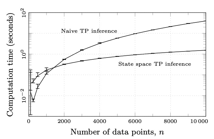
<p>The first experiment demonstrates the speed advantage of the state-space formulation. Instead of building and factorizing the full covariance matrix, the model updates a compact latent state sequentially. This is where the linear-time scaling becomes visible in practice.</p>

<p><img src="/images/blog/ss-tp/figure1.png" alt="" /></p>

<p><em>Figure 1: computational efficiency of naive inference versus the state-space method.</em></p>

<h3 id="experiment-2-robustness-on-synthetic-and-real-data">Experiment 2: robustness on synthetic and real data</h3>

<p>The second experiment compares several data regimes:</p>

<ul>
  <li><strong>Synth A</strong>: Gaussian noise,</li>
  <li><strong>Synth B</strong>: Student-t noise,</li>
  <li><strong>Synth C</strong>: a mixture with outliers,</li>
  <li><strong>Electricity</strong>: hourly household electricity consumption,</li>
  <li><strong>Stock (Apple)</strong>: log-prices over a long time span.</li>
</ul>

<p>These settings test both accuracy and robustness. On clean Gaussian data, the GP and TP behave similarly. On contaminated data, the Student-t model is more stable and produces more meaningful uncertainty estimates.</p>

<p><img src="/images/blog/ss-tp/figure2.png" alt="" /></p>

<p><em>Figure 2: comparison of naive and state-space inference for GP and TP, with average MSE and log-likelihood.</em></p>

<h3 id="experiment-3-missing-data-interpolation">Experiment 3: missing data interpolation</h3>

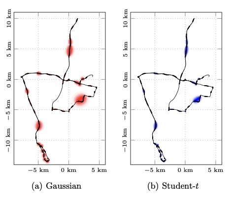
<p>A particularly useful application is interpolation of missing or unreliable measurements. In such settings, the Student-t process is usually more conservative around suspicious regions and more confident elsewhere, which improves reconstruction quality.</p>

<p><img src="/images/blog/ss-tp/figure3.png" alt="" /></p>

<p><em>Figure 3: interpolation of missing observations with wider uncertainty around corrupted regions.</em></p>

<h2 id="conclusion">Conclusion</h2>

<p>Student-t process regression gives a simple but powerful upgrade over standard Gaussian-process regression:</p>

<ul>
  <li>it keeps the Bayesian, analytical nature of GP inference;</li>
  <li>it reacts to outliers through adaptive uncertainty;</li>
  <li>and, with a state-space representation, it becomes scalable enough for long time series and online inference.</li>
</ul>

<p>The main message is that robustness and efficiency do not have to be in conflict. By combining heavy-tailed probabilistic modeling with Kalman-style inference, we get a method that is practical for real data and still mathematically elegant.</p>

<p><strong>Main takeaways</strong></p>

<ul>
  <li><strong>GPs are elegant but brittle</strong> when the data contains outliers.</li>
  <li><strong>Student-t processes add robustness</strong> through heavy tails and observation-dependent uncertainty.</li>
  <li><strong>State-space inference makes the method scalable</strong>, turning $O(n^3)$ inference into an approximately linear-time algorithm for temporal kernels.</li>
  <li><strong>Filtering and smoothing remain analytical</strong>, so the model stays interpretable and easy to optimize.</li>
</ul>]]></content><author><name>Stepanov Ilya</name></author><category term="Gaussian processes" /><category term="Student-t processes" /><category term="State-space models" /><category term="Kalman filtering" /><summary type="html"><![CDATA[Based on the state-space regression framework for Student-t processes.]]></summary></entry><entry xml:lang="en"><title type="html">Multi-Task Learning as Multi-Objective Optimization</title><link href="https://intsystems.github.io/materials/blog/mgda/" rel="alternate" type="text/html" title="Multi-Task Learning as Multi-Objective Optimization" /><published>2026-05-15T00:00:00+00:00</published><updated>2026-05-15T00:00:00+00:00</updated><id>https://intsystems.github.io/materials/blog/mgda</id><content type="html" xml:base="https://intsystems.github.io/materials/blog/mgda/"><![CDATA[<p><strong>Based on the 2018 NeurIPS conference paper by Ozan Sener and Vladlen Koltun</strong></p>

<p><em>If you find this topic interesting, please check out the <a href="https://papers.nips.cc/paper/2018/file/432aca3a1e345e339f35a30c8f65edce-Paper.pdf">original paper</a>!</em></p>

<h2 id="introduction">Introduction</h2>

<p>In the realm of statistics, there is a fascinating phenomenon known as <strong>Stein’s Paradox</strong>. It states that when you need to estimate the means of three or more Gaussian random variables, you actually get a better estimate if you compute them <em>jointly</em> using samples from all of them, rather than estimating each one separately—even if the variables are completely independent!</p>

<p>This mathematical quirk serves as an early motivation for <strong>Multi-Task Learning (MTL)</strong>. In modern machine learning, MTL leverages the shared inductive bias across different tasks to improve overall performance. For instance, in autonomous driving, predicting depth and segmenting pedestrians are seemingly different tasks, yet they are governed by the same physical laws of optics and scene geometry. Why learn the rules of the visual world from scratch for every single task when you can learn them once and share the knowledge?</p>

<h3 id="the-problem-with-the-standard-approach">The Problem with the Standard Approach</h3>

<p>Typically, MTL in deep neural networks is implemented via hard parameter sharing: the network has shared parameters $\theta^{sh}$ (the feature extractor/encoder) and task-specific parameters $\theta^{t}$ (the heads/decoders).</p>

<p>The most common way to optimize such a model is by taking a <strong>linear combination of empirical losses</strong>:</p>

\[\min_{\theta^{sh}, \theta^{1}, \dots, \theta^{T}} \sum_{t=1}^{T} c_t \hat{\mathcal{L}}^t(\theta^{sh}, \theta^t)\]

<p>where $c_t$ are static or dynamically computed weights.</p>

<p><span style="color:red"><strong>The flaw:</strong></span> This approach makes a massive assumption—that the tasks do not compete. In reality, tasks frequently conflict. Improving the loss for task A might degrade the loss for task B. When tasks compete, the linear combination forces an arbitrary trade-off, usually requiring an excruciatingly expensive grid search over the weights $c_t$ to find a “good enough” balance.</p>

<h2 id="the-paradigm-shift-multi-objective-optimization">The Paradigm Shift: Multi-Objective Optimization</h2>

<p>Instead of forcing tasks to cooperate through a weighted sum, Sener and Koltun propose casting MTL explicitly as <strong>Multi-Objective Optimization (MOO)</strong>. In MOO, we accept that tasks conflict and that a single “global optimum” that minimizes all losses simultaneously simply might not exist.</p>

<p>Instead, the goal is to find an optimal trade-off, mathematically defined as a <strong>Pareto optimal</strong> solution.</p>

<h3 id="pareto-optimality-defined">Pareto Optimality Defined</h3>

<p>To understand the objective, we must define two key concepts:</p>
<ol>
  <li><strong>Dominance:</strong> A set of parameters $\theta$ <em>dominates</em> another set $\bar{\theta}$ if it is better or equal on <em>all</em> tasks, and strictly better on at least one task. Mathematically: $\forall t, \hat{\mathcal{L}}^t(\theta) \leq \hat{\mathcal{L}}^t(\bar{\theta})$ and $\exists i \text{ s.t. } \hat{\mathcal{L}}^i(\theta) &lt; \hat{\mathcal{L}}^i(\bar{\theta})$.</li>
  <li><strong>Pareto Optimality:</strong> A solution $\theta^\ast$ is <em>Pareto optimal</em> if no other solution dominates it. The set of all such solutions forms the <strong>Pareto front</strong>.</li>
</ol>

<p>Our new objective is to use gradient-based algorithms to smoothly navigate our model parameters until we land on this Pareto front.</p>

<h2 id="the-math-mgda-and-kkt-conditions">The Math: MGDA and KKT Conditions</h2>

<p>To achieve Pareto optimality, the authors turn to the <strong>Multiple Gradient Descent Algorithm (MGDA)</strong>. MGDA relies on the Karush-Kuhn-Tucker (KKT) conditions for multi-objective optimization.</p>

<p>For a point to be Pareto stationary, two conditions must hold:</p>
<ol>
  <li>For task-specific parameters: $\nabla_{\theta^{t}} \hat{\mathcal{L}}^t(\theta^{sh}, \theta^t) = 0$</li>
  <li>For shared parameters: there must exist weights $\alpha_1, \dots, \alpha_T \geq 0$ where $\sum_{t=1}^T \alpha_t = 1$, such that:
\(\sum_{t=1}^T \alpha_t \nabla_{\theta^{sh}} \hat{\mathcal{L}}^t(\theta^{sh}, \theta^t) = 0\)</li>
</ol>

<p>To satisfy the second condition and find a gradient direction that improves <em>all</em> tasks simultaneously, we must solve an optimization problem on a simplex at each training step:</p>

\[\min_{\alpha_1, \dots, \alpha_T} \left\| \sum_{t=1}^T \alpha_t \nabla_{\theta^{sh}} \hat{\mathcal{L}}^t(\theta^{sh}, \theta^t) \right\|_2^2 \quad s.t. \sum_{t=1}^T \alpha_t = 1, \alpha_t \geq 0\]

<p>Geometrically, this is equivalent to finding the minimum-norm point within the convex hull of the task gradients. If you think of each task as a player in a multi-directional tug-of-war over the shared weights, this algorithm calculates the exact center of force where everyone is satisfied.</p>

<h2 id="the-computational-bottleneck">The Computational Bottleneck</h2>

<p>Here is where the elegant theory hits a brick wall of computational reality.</p>

<p>To solve the simplex optimization problem above, we need the gradient of <em>each</em> task’s loss with respect to the <em>shared</em> parameters: $\nabla_{\theta^{sh}} \hat{\mathcal{L}}^t$. 
In a deep neural network, computing this requires a separate backward pass for each task. If you have 40 tasks, you need <strong>40 backward passes per training step</strong>. This linear scaling with the number of tasks makes standard MGDA entirely impractical for deep learning.</p>

<h3 id="the-proposed-solution-mgda-ub">The Proposed Solution: MGDA-UB</h3>

<p>To bypass this bottleneck, the authors exploit the architecture of neural networks. Let $Z = g(x; \theta^{sh})$ be the shared representations (the output of the shared encoder).</p>

<p>Using the chain rule, we can extract the Jacobian of the representation w.r.t the shared parameters: $\frac{\partial Z}{\partial \theta^{sh}}$. The authors prove the following upper bound:</p>

\[\left\| \sum_{t=1}^T \alpha_t \nabla_{\theta^{sh}} \hat{\mathcal{L}}^t \right\|_2^2 \leq \left\| \frac{\partial Z}{\partial \theta^{sh}} \right\|_2^2 \left\| \sum_{t=1}^T \alpha_t \nabla_{Z} \hat{\mathcal{L}}^t \right\|_2^2\]

<p>Notice something beautiful here? The term $\left| \frac{\partial Z}{\partial \theta^{sh}} \right|_2^2$ <strong>does not depend on $\alpha$</strong>.</p>

<p>This means to find the optimal $\alpha$ weights, we can drop the expensive shared-parameter gradients and optimize <em>only</em> using the gradients with respect to the representations $Z$:</p>

\[\min_{\alpha} \left\| \sum_{t=1}^T \alpha_t \nabla_{Z} \hat{\mathcal{L}}^t \right\|_2^2\]

<p><strong>Why is this a game-changer?</strong> The gradients with respect to $Z$ ($\nabla_{Z} \hat{\mathcal{L}}^t$) can be computed for all tasks simultaneously in a <strong>single backward pass</strong>. The computational overhead of MOO effectively drops to zero.</p>

<p>The authors theoretically guarantee this approach with a theorem:</p>
<blockquote>
  <p><strong>Theorem 1:</strong> Assuming $\frac{\partial Z}{\partial \theta^{sh}}$ is full rank, if $\alpha^{1,\dots,T}$ is the solution to the MGDA-UB problem, it will either yield a Pareto stationary point or provide a descent direction that strictly decreases all objective losses.</p>
</blockquote>

<h3 id="the-final-algorithm">The Final Algorithm</h3>

<p>The training loop elegantly comes together as follows:</p>
<ol>
  <li>Update task-specific parameters $\theta^t$ using their respective gradients.</li>
  <li>Compute the gradients of task losses with respect to the shared representations $Z$.</li>
  <li>Solve the Frank-Wolfe optimization algorithm on the simplex to find the optimal $\alpha$ weights.</li>
  <li>Calculate the common descent direction $\Delta = \sum_{t=1}^T \alpha_t \nabla_{\theta^{sh}} \hat{\mathcal{L}}^t$ (effectively done via a standard backward pass weighted by $\alpha$).</li>
  <li>Update shared parameters $\theta^{sh}$ using $\Delta$.</li>
</ol>

<hr />

<h2 id="experimental-results">Experimental Results</h2>

<p>To prove that this isn’t just theoretical wizardry, the authors evaluated MGDA-UB on three distinct benchmarks, increasing the complexity and the number of tasks.</p>

<h3 id="1-multimnist-capacity-competition">1. MultiMNIST (Capacity Competition)</h3>

<p>The first experiment uses MultiMNIST, where two digits are overlaid on a single image. The two tasks are classifying the top-left digit and the bottom-right digit.</p>

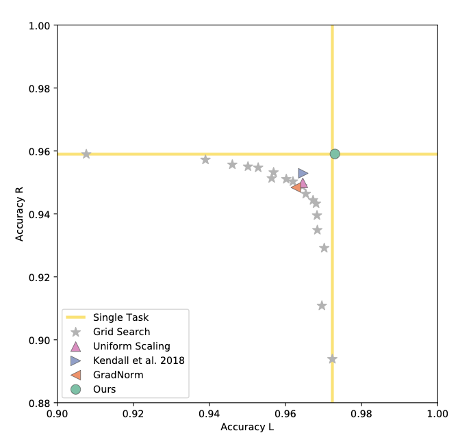
<p>Because the network has limited capacity, these two tasks heavily compete. As seen in the results, standard linear combinations (even after exhaustive grid search) fail to match the performance of training two entirely separate models (Single Task).</p>

<p>MGDA-UB, however, perfectly navigates the capacity competition, matching single-task performance without needing two separate networks.</p>

<h6 id="figure-1-authors-plot-the-obtained-accuracy-in-detecting-the-left-and-right-digits-for-all-baselines-the-grid-search-results-suggest-that-the-tasks-compete-for-model-capacity-proposed-method-is-the-only-one-that-finds-a-solution-that-is-as-good-as-training-a-dedicated-model-for-each-task-top-right-is-better">Figure 1. Authors plot the obtained accuracy in detecting the left and right digits for all baselines. The grid-search results suggest that the tasks compete for model capacity. Proposed method is the only one that finds a solution that is as good as training a dedicated model for each task. Top-right is better.</h6>
<p><em><img src="/images/blog/mgda/multimnist.png" alt="Placeholder: Figure 3 from paper - MultiMNIST Accuracy Profile" /></em></p>

<h6 id="table-1-comparison-of-proposed-method-vs-baselines-on-multimnist">Table 1. Comparison of proposed method vs baselines on MultiMNIST.</h6>

<table>
  <thead>
    <tr>
      <th style="text-align: left">Method</th>
      <th style="text-align: center">Left digit acc. $\uparrow$</th>
      <th style="text-align: center">Right digit acc. $\uparrow$</th>
    </tr>
  </thead>
  <tbody>
    <tr>
      <td style="text-align: left">Single task</td>
      <td style="text-align: center">97.23</td>
      <td style="text-align: center"><strong>95.90</strong></td>
    </tr>
    <tr>
      <td style="text-align: left">Uniform scaling</td>
      <td style="text-align: center">96.46</td>
      <td style="text-align: center">94.99</td>
    </tr>
    <tr>
      <td style="text-align: left">Kendall et al. 2018</td>
      <td style="text-align: center">96.47</td>
      <td style="text-align: center">95.29</td>
    </tr>
    <tr>
      <td style="text-align: left">GradNorm</td>
      <td style="text-align: center">96.27</td>
      <td style="text-align: center">94.84</td>
    </tr>
    <tr>
      <td style="text-align: left"><strong>Ours (MGDA-UB)</strong></td>
      <td style="text-align: center"><strong>97.26</strong></td>
      <td style="text-align: center"><strong>95.90</strong></td>
    </tr>
  </tbody>
</table>

<h3 id="2-celeba-scaling-to-40-tasks">2. CelebA (Scaling to 40 Tasks)</h3>

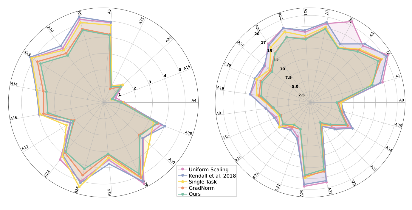
<p>To test scalability, the authors framed the CelebA facial attribute dataset as a 40-way multi-label classification problem. Grid search is mathematically impossible here.</p>

<p>Despite the massive number of tasks, MGDA-UB seamlessly scaled to 40 objectives, beating Uniform Scaling, Uncertainty Weighting (Kendall et al.), and GradNorm, achieving the lowest average error.</p>

<h6 id="figure-2-radar-charts-of-percentage-error-per-attribute-on-celeba-lower-is-better-authors-divide-attributes-into-two-sets-for-legibility-easy-on-the-left-hard-on-the-right-zoom-in-for-details">Figure 2. Radar charts of percentage error per attribute on CelebA. Lower is better. Authors divide attributes into two sets for legibility: easy on the left, hard on the right. Zoom in for details.</h6>

<p><em><img src="/images/blog/mgda/celeba.png" alt="Placeholder: Figure 2 from paper - Radar charts of percentage error per attribute on CelebA" /></em></p>

<h6 id="table-2-comparison-of-proposed-method-vs-baselines-on-celeba">Table 2. Comparison of proposed method vs baselines on CelebA.</h6>

<table>
  <thead>
    <tr>
      <th style="text-align: left">Method</th>
      <th style="text-align: center">Average error $\downarrow$</th>
    </tr>
  </thead>
  <tbody>
    <tr>
      <td style="text-align: left">Single task</td>
      <td style="text-align: center">8.77</td>
    </tr>
    <tr>
      <td style="text-align: left">Uniform scaling</td>
      <td style="text-align: center">9.62</td>
    </tr>
    <tr>
      <td style="text-align: left">Kendall et al. 2018</td>
      <td style="text-align: center">9.53</td>
    </tr>
    <tr>
      <td style="text-align: left">GradNorm</td>
      <td style="text-align: center">8.44</td>
    </tr>
    <tr>
      <td style="text-align: left"><strong>Ours (MGDA-UB)</strong></td>
      <td style="text-align: center"><strong>8.25</strong></td>
    </tr>
  </tbody>
</table>

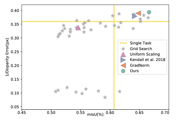
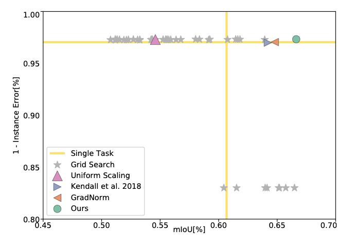
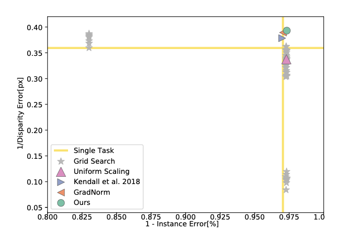
<h3 id="3-cityscapes-complex-scene-understanding">3. Cityscapes (Complex Scene Understanding)</h3>

<p>Moving to a real-world autonomous driving analog, the model was tasked with jointly performing semantic segmentation, instance segmentation, and monocular depth estimation on the Cityscapes dataset using a ResNet-50 encoder.</p>

<p>Once again, MGDA-UB achieved state-of-the-art results across all three metrics. It allowed the tasks to actively cooperate, beating single-task baselines across the board.</p>

<h6 id="figure-3-authors-plot-the-performance-of-all-baselines-for-the-tasks-of-semantic-segmentation-instance-segmentation-and-depth-estimation-they-use-miou-for-semantic-segmentation-error-of-per-pixel-regression-normalized-to-image-size-for-instance-segmentation-and-disparity-error-for-depth-estimation-to-convert-errors-to-performance-measures-they-use-1---instance-error-and-1disparity-error-they-plot-2d-projections-of-the-performance-profile-for-each-pair-of-tasks-although-they-plot-pairwise-projections-for-visualization-each-point-in-the-plots-solves-all-tasks-top-right-is-better">Figure 3. Authors plot the performance of all baselines for the tasks of semantic segmentation, instance segmentation, and depth estimation. They use mIoU for semantic segmentation, error of per-pixel regression (normalized to image size) for instance segmentation, and disparity error for depth estimation. To convert errors to performance measures, they use 1 - instance error and 1/disparity error. They plot 2D projections of the performance profile for each pair of tasks. Although they plot pairwise projections for visualization, each point in the plots solves all tasks. Top-right is better.</h6>

<p><img src="/images/blog/mgda/cityscapes_1.png" alt="CS1" />
<img src="/images/blog/mgda/cityscapes_2.png" alt="CS2" /> 
<img src="/images/blog/mgda/cityscapes_3.png" alt="CS3" /></p>

<h3 id="4-the-role-of-the-approximation-ablation-study">4. The Role of the Approximation (Ablation Study)</h3>

<p>A crucial question remains: Does approximating the true MGDA with the Upper Bound (MGDA-UB) hurt performance?</p>

<p>The authors compared exact MGDA (multiple backward passes) against MGDA-UB. The results were startling. On CelebA (40 tasks), the training time dropped from <strong>42.9 hours to just 1.6 hours</strong> (a ~25x speedup).</p>

<p>Even more surprisingly, <strong>accuracy slightly improved</strong> with the approximation. The authors hypothesize that calculating the simplex optimization in the lower-dimensional space of $Z$ (thousands of dimensions) rather than $\theta^{sh}$ (millions of dimensions) significantly reduces gradient noise, leading to higher stability.</p>

<table>
  <thead>
    <tr>
      <th style="text-align: left">Method</th>
      <th style="text-align: center">Time (h) $\downarrow$</th>
      <th style="text-align: center">Segm mIoU $\uparrow$</th>
      <th style="text-align: center">Inst err $\downarrow$</th>
      <th style="text-align: center">Disp err $\downarrow$</th>
      <th style="text-align: center">Time (h) $\downarrow$</th>
      <th style="text-align: center">Avg err $\downarrow$</th>
    </tr>
  </thead>
  <tbody>
    <tr>
      <td style="text-align: left"> </td>
      <td style="text-align: center"><strong>Scene (3 tasks)</strong></td>
      <td style="text-align: center"> </td>
      <td style="text-align: center"> </td>
      <td style="text-align: center"> </td>
      <td style="text-align: center"><strong>CelebA (40 tasks)</strong></td>
      <td style="text-align: center"> </td>
    </tr>
    <tr>
      <td style="text-align: left">Exact MGDA</td>
      <td style="text-align: center">66.1</td>
      <td style="text-align: center">66.13</td>
      <td style="text-align: center">10.28</td>
      <td style="text-align: center">2.59</td>
      <td style="text-align: center">42.9</td>
      <td style="text-align: center">8.33</td>
    </tr>
    <tr>
      <td style="text-align: left"><strong>MGDA-UB</strong></td>
      <td style="text-align: center"><strong>38.6</strong></td>
      <td style="text-align: center"><strong>66.63</strong></td>
      <td style="text-align: center"><strong>10.25</strong></td>
      <td style="text-align: center"><strong>2.54</strong></td>
      <td style="text-align: center"><strong>1.6</strong></td>
      <td style="text-align: center"><strong>8.25</strong></td>
    </tr>
  </tbody>
</table>

<hr />

<h2 id="conclusion">Conclusion</h2>

<p>Sener and Koltun’s paper shifts the paradigm of Multi-Task Learning from empirical weight guessing to rigorous mathematical optimization.</p>

<p><strong>Key Takeaways:</strong></p>
<ol>
  <li><strong>Mathematically Sound:</strong> Formulating MTL as finding a Pareto optimum removes the need for heuristic weight tuning.</li>
  <li><strong>Highly Scalable:</strong> The MGDA-UB upper bound reduces an $O(T)$ backward pass bottleneck to a single backward pass, making gradient-based MOO practical for massive deep neural networks.</li>
  <li><strong>Theoretically Proven:</strong> Optimizing the upper bound is mathematically guaranteed to yield a Pareto stationary point (under full-rank Jacobian assumptions).</li>
  <li><strong>State-of-the-Art:</strong> It efficiently utilizes shared model capacity, achieving top performance across digit classification, multi-label prediction (up to 40 tasks), and dense computer vision tasks.</li>
</ol>]]></content><author><name>Altay Eynullayev</name></author><category term="Multi-Task Learning" /><category term="Multi-Objective Optimization" /><category term="Pareto Optimality" /><category term="BMM" /><summary type="html"><![CDATA[Based on the 2018 NeurIPS conference paper by Ozan Sener and Vladlen Koltun]]></summary></entry><entry xml:lang="en"><title type="html">Score-Based VAMP with Fisher-Information-Based Onsager Correction</title><link href="https://intsystems.github.io/materials/blog/scvamp-minashkin/" rel="alternate" type="text/html" title="Score-Based VAMP with Fisher-Information-Based Onsager Correction" /><published>2026-05-14T00:00:00+00:00</published><updated>2026-05-14T00:00:00+00:00</updated><id>https://intsystems.github.io/materials/blog/scvamp_minashkin</id><content type="html" xml:base="https://intsystems.github.io/materials/blog/scvamp-minashkin/"><![CDATA[<p><strong>Based on the 2026 paper by Tadashi Wadayama and Takumi Takahashi</strong></p>

<p><em>If you find this topic interesting, please check out the <a href="https://arxiv.org/abs/2601.07095">original paper</a>!</em></p>

<h2 id="introduction">Introduction</h2>

<p><strong>Vector Approximate Message Passing (VAMP)</strong> is one of the cornerstones of modern high-dimensional statistical inference. Rooted in the statistical physics of spin glasses, VAMP and its predecessor AMP provide iterative algorithms for solving linear inverse problems of the form $\mathbf{y} = \mathbf{A}\mathbf{x}_0 + \mathbf{w}$. Their key feature is the <strong>Onsager correction</strong> — a seemingly mysterious term that removes harmful correlations between iterations and ensures that the algorithm’s dynamics can be exactly tracked by <strong>State Evolution (SE)</strong> in the large-system limit. When the priors and likelihoods are Gaussian, VAMP achieves Bayes-optimal performance.</p>

<p>However, classical VAMP faces a critical bottleneck when we try to apply it to real-world problems. The Onsager correction requires computing the <strong>divergence</strong> (trace of the Jacobian) of the denoiser $\eta_t(\cdot)$ at every iteration:
\(\alpha_t = \frac{1}{N}\operatorname{div}(\eta_t) = \frac{1}{N}\sum_{i=1}^N \frac{\partial \eta_{t,i}}{\partial r_i}.\)</p>

<p>For simple denoisers (e.g., soft-thresholding) this is trivial. But for <strong>deep neural network denoisers</strong> — the kind that actually work well on natural images, medical imaging, or scientific data — computing this divergence via automatic differentiation is prohibitively expensive. It costs $\mathcal{O}(N^2)$ operations or requires memory-hungry Monte Carlo approximations, effectively negating the computational advantages of message passing.</p>

<p>In their 2026 paper, Wadayama and Takahashi propose <strong>Score-based VAMP (SC-VAMP)</strong>, a elegant reformulation that eliminates the Jacobian entirely. The key insight is that both the optimal denoiser <em>and</em> its Onsager correction can be expressed purely in terms of the <strong>score function</strong> $\nabla \log p(\mathbf{r})$ and the <strong>Fisher information</strong> $\mathbb{E}[|\nabla \log p(\mathbf{r})|^2]$. Since score functions are exactly what modern diffusion models learn, SC-VAMP turns any pre-trained score network into a Bayes-optimal inverse problem solver — without ever computing a derivative of the network.</p>

<h2 id="background-from-amp-to-vamp">Background: From AMP to VAMP</h2>

<p><strong>AMP</strong> (Approximate Message Passing) is an iterative algorithm for linear inverse problems that alternates between a linear step and a nonlinear denoising step, with the Onsager correction subtracting the “self-interaction” of the iterate. Its asymptotic dynamics are exactly characterized by SE, a scalar recursion tracking the mean-square error.</p>

<p><strong>VAMP</strong> generalizes AMP to handle matrices $\mathbf{A}$ of arbitrary singular value distributions (not just i.i.d. sub-Gaussian ones). It does so by using the SVD of $\mathbf{A}$ and maintaining two modules:</p>
<ul>
  <li><strong>Module A (LMMSE):</strong> processes the linear observations $\mathbf{y} = \mathbf{A}\mathbf{x} + \mathbf{w}$.</li>
  <li><strong>Module B (Denoiser):</strong> applies a nonlinear estimator $\eta(\mathbf{r})$ to remove noise.</li>
</ul>

<p>The Achilles’ heel is the divergence computation in Module B. For a neural denoiser with millions of parameters, $\operatorname{div}(\eta)$ is a nightmare.</p>

<h2 id="method-score-based-vamp">Method: Score-Based VAMP</h2>

<p>SC-VAMP resolves this by re-parameterizing the entire algorithm in terms of the score function. The paper makes three interconnected contributions.</p>

<h3 id="tweedies-formula-and-the-score-function">Tweedie’s Formula and the Score Function</h3>

<p>Suppose we observe a noisy vector $\mathbf{r} = \mathbf{x} + \gamma^{-1/2}\mathbf{z}$ where $\mathbf{z} \sim \mathcal{N}(\mathbf{0}, \mathbf{I})$. The optimal MMSE denoiser is given by <strong>Tweedie’s formula</strong>:
\(\hat{\mathbf{x}} = \mathbb{E}[\mathbf{x}|\mathbf{r}] = \mathbf{r} + \frac{1}{\gamma}\nabla_{\mathbf{r}} \log p(\mathbf{r}; \gamma).\)</p>

<p>The gradient term is the $\textbf{score function}$. Modern diffusion models train neural networks 
$\mathbf{s}<em>\theta(\mathbf{r}, \gamma) \approx \nabla</em>{\mathbf{r}} \log p(\mathbf{r}; \gamma)$. 
Thus, we can implement the optimal denoiser using only a forward pass through a score network:
\(\mathbf{x}_{\text{post}} = \mathbf{r} + \frac{1}{\gamma} \mathbf{s}_\theta(\mathbf{r}, \gamma),\)
where $\gamma$ is the inverse input variance (so that $v_{\text{in}} = \gamma^{-1}$).</p>

<h3 id="jacobian-free-onsager-correction-via-fisher-information">Jacobian-Free Onsager Correction via Fisher Information</h3>

<p>Here is the theoretical centerpiece of the paper. The authors prove that the Onsager coefficient $\alpha(v_{\text{in}})$, which normally requires the divergence of the denoiser, can be computed directly from the <strong>conditional Fisher information</strong>:
\(\alpha(v_{\text{in}}) = 1 - \frac{v_{\text{in}}}{N} J(\gamma),\)
where
\(J(\gamma) = \mathbb{E}_{\mathbf{r}}\left[\left\|\nabla_{\mathbf{r}} \log p(\mathbf{r}; \gamma)\right\|^2\right] = \mathbb{E}_{\mathbf{r}}\left[\left\|\mathbf{s}_\theta(\mathbf{r}, \gamma)\right\|^2\right].\)</p>

<p>In other words: the Onsager correction is determined by the expected squared norm of the score function. No Jacobians. No backpropagation through the denoiser. Just evaluate the score network on a mini-batch, average the squared $\ell_2$-norms, and plug into the formula.</p>

<p>The paper provides multiple derivations of this identity — via <strong>Stein’s identity</strong>, via the <strong>I-MMSE relationship</strong> (de Bruijn’s identity), and via the information-geometric interpretation of the Onsager term as a “curvature correction” governed by the local Fisher information.</p>

<h3 id="the-sc-vamp-algorithm">The SC-VAMP Algorithm</h3>

<p>Putting it together, one iteration of SC-VAMP looks like this:</p>

<ol>
  <li><strong>LMMSE step (Module A):</strong> Update using linear measurements (standard VAMP).</li>
  <li><strong>Denoising step (Module B):</strong>
\(\mathbf{x}_{1,t} = \mathbf{r}_{1,t} + v_{1,t} \mathbf{s}_\theta(\mathbf{r}_{1,t}, v_{1,t}).\)</li>
  <li><strong>Onsager correction:</strong>
\(\alpha_{1,t} = 1 - \frac{v_{1,t}}{N} \hat{J}_\theta, \quad \hat{J}_\theta = \frac{1}{B}\sum_{i=1}^B \|\mathbf{s}_\theta(\mathbf{r}_{1,t}^{(i)})\|^2.\)</li>
  <li><strong>Extrinsic output:</strong>
\(\mathbf{r}_{2,t} = \frac{\mathbf{x}_{1,t} - \alpha_{1,t}\mathbf{r}_{1,t}}{1 - \alpha_{1,t}}.\)</li>
</ol>

<p>The algorithm is <strong>Jacobian-free</strong>: the only operation involving the neural network is a forward pass to get the score. This reduces the per-iteration cost by a factor of <strong>10–50×</strong> compared to standard VAMP with AutoDiff-based divergence computation.</p>

<h3 id="using-pre-trained-denoisers">Using Pre-Trained Denoisers</h3>

<p>A practical bonus: if you already have a state-of-the-art denoiser $\eta_{\text{opt}}(\cdot)$ (e.g., DnCNN, DRUNet) but no explicit score model, you can extract an <em>implicit score</em> via Tweedie’s formula:
\(\hat{\mathbf{s}}(\mathbf{r}) = \frac{\eta_{\text{opt}}(\mathbf{r}) - \mathbf{r}}{v_{\text{in}}}.\)</p>

<p>Substituting this into the Fisher information estimator yields a fully plug-and-play Onsager correction, letting SC-VAMP leverage existing denoiser libraries without retraining.</p>

<h2 id="theoretical-guarantees">Theoretical Guarantees</h2>

<p>The paper demonstrates that SC-VAMP is not just a computational hack — it is theoretically sound.</p>

<h3 id="optimality-in-scalar-gaussian-channels">Optimality in Scalar Gaussian Channels</h3>

<p><strong>Theorem 1</strong> shows that in the classical linear Gaussian setting, SC-VAMP reduces exactly to standard Bayes-optimal VAMP. For a scalar channel $Y = X + Z$ with $X \sim \mathcal{N}(0, P)$ and $Z \sim \mathcal{N}(0, \sigma^2)$, the SE fixed point of SC-VAMP achieves the mutual information:
\(I_{\text{VAMP}} = I(X;Y) = \frac{1}{2}\log\left(1 + \frac{P}{\sigma^2}\right).\)</p>

<p>Moreover, the point estimate converges to the Wiener filter $\hat{x} = \frac{P}{P+\sigma^2}y$. Thus, SC-VAMP preserves the optimality of VAMP exactly where VAMP is already optimal.</p>

<h3 id="state-evolution-and-decoupling">State Evolution and Decoupling</h3>

<p>The authors verify empirically that the MSE trajectory of SC-VAMP follows the theoretical SE prediction precisely:</p>

<p><img src="images/blog/scvamp_minashkin/fig1.png" alt="" />
<em><strong>Figure 1:</strong> MSE convergence of SC-VAMP (blue) versus State Evolution theory (red dashed). The trajectories are indistinguishable, confirming that the Fisher-information-based Onsager correction is unbiased.</em></p>

<p>This confirms that the score-norm approximation does not break the decoupling principle. The algorithm still decomposes the high-dimensional problem into independent scalar Gaussian channels in the large-system limit.</p>

<h3 id="information-theoretic-perspective">Information-Theoretic Perspective</h3>

<p>Perhaps the most conceptually rich part of the paper is the connection to the <strong>entropic Central Limit Theorem</strong>. The authors interpret the linear mixing step in VAMP as a “Gaussianizer”: each iteration reduces the non-Gaussianity (in KL-divergence) of the estimation error. This provides an information-theoretic justification for why the Gaussian approximation underlying SE remains valid even beyond idealized i.i.d. settings, including nonlinear regimes.</p>

<h2 id="experiments">Experiments</h2>

<p>The experimental section focuses on a linear observation system with a Bernoulli-Gaussian prior ($N=2000$, $M=1000$, $\rho=0.1$, SNR = 20 dB). The score function is learned via denoising score matching (DSM).</p>

<h3 id="mse-and-convergence">MSE and Convergence</h3>

<p>As shown in Figure 1, SC-VAMP tracks the theoretical SE curve almost perfectly. The algorithm converges to the same fixed point as classical VAMP with exact divergence, but with drastically lower computational cost.</p>

<h3 id="exit-chart-analysis">EXIT Chart Analysis</h3>

<p><img src="images/blog/scvamp_minashkin/fig2.png" alt="" />
<em><strong>Figure 2:</strong> EXIT-style analysis showing Module A (observation) and Module B (denoiser) transfer characteristics. The SE trajectory (green) and actual SC-VAMP trajectory (gray dashed) follow the characteristic curves and converge to the same fixed point.</em></p>
<p>The EXIT chart confirms that the score-based SISO modules correctly implement the MMSE estimator and that the mini-batch Fisher information estimator provides an accurate Onsager term.</p>

<h2 id="extensions-and-future-directions">Extensions and Future Directions</h2>

<p>The paper sketches several promising extensions:</p>

<ul>
  <li><strong>Random orthogonal/unitary mixing:</strong> To handle structured or correlated sensing matrices (where standard VAMP/AMP often fails), SC-VAMP can be combined with random rotations that “whiten” the problem.</li>
  <li><strong>Nonlinear observations:</strong> The score-based formalism extends naturally to $\mathbf{y} = f(\mathbf{x}) + \mathbf{w}$ with deterministic nonlinearities $f$, such as sensor saturation or optical systems.</li>
  <li><strong>Flow matching:</strong> The authors note that since score functions and velocity fields are algebraically equivalent under a given probability path, an SC-VAMP-like algorithm could be built using rectified flow or flow matching networks — potentially offering more stable training in low-noise regimes.</li>
</ul>

<h2 id="conclusion">Conclusion</h2>

<p>SC-VAMP represents a significant step in unifying classical statistical-physics-based inference with modern deep learning. By reformulating the denoiser and its Onsager correction entirely through the lens of score functions and Fisher information, it eliminates the Jacobian bottleneck that has long plagued neural AMP/VAMP methods.</p>

<p><strong>Main strengths of SC-VAMP:</strong></p>
<ul>
  <li><strong>Jacobian-free:</strong> The Onsager correction requires only the squared norm of the score network output, enabling 10–50× speedup per iteration.</li>
  <li><strong>Plug-and-play:</strong> Works with any pre-trained score model or denoiser; no retraining or architectural constraints.</li>
  <li><strong>Theoretically grounded:</strong> Recovers exact Bayes-optimal VAMP in Gaussian settings and tracks State Evolution perfectly.</li>
  <li><strong>Universal:</strong> Extends to nonlinear observations, complex priors, and structured sensing matrices.</li>
</ul>

<p><strong>Limitations:</strong></p>
<ul>
  <li><strong>Decoupling assumption:</strong> Like all AMP/VAMP variants, SC-VAMP relies on asymptotic statistical decoupling; for highly structured finite-dimensional problems, the Gaussian approximation may be less accurate.</li>
  <li><strong>Score estimation quality:</strong> The method inherits any bias or variance from the learned score network. In low-noise regimes, score matching can be unstable (though flow-matching extensions may remedy this).</li>
  <li><strong>Mini-batch variance:</strong> The Fisher information is estimated via Monte Carlo; very small batch sizes could introduce variance into the Onsager term.</li>
</ul>

<p>SC-VAMP is a rare example of a method that is simultaneously cheaper, more general, and theoretically cleaner than its predecessor. It opens the door to applying message-passing algorithms to the complex, black-box inference problems that arise in computational imaging, scientific computing, and beyond.</p>]]></content><author><name>Vladislav Minashkin</name></author><category term="Approximate Message Passing" /><category term="Score-based models" /><category term="Inverse problems" /><category term="BMM" /><summary type="html"><![CDATA[Based on the 2026 paper by Tadashi Wadayama and Takumi Takahashi]]></summary></entry><entry xml:lang="en"><title type="html">When Gaussian Processes Meet the Ensemble Kalman Filter</title><link href="https://intsystems.github.io/materials/blog/rubtsov-gaussian-process-and-kalman-filter/" rel="alternate" type="text/html" title="When Gaussian Processes Meet the Ensemble Kalman Filter" /><published>2026-05-14T00:00:00+00:00</published><updated>2026-05-14T00:00:00+00:00</updated><id>https://intsystems.github.io/materials/blog/rubtsov_gaussian_process_and_kalman_filter</id><content type="html" xml:base="https://intsystems.github.io/materials/blog/rubtsov-gaussian-process-and-kalman-filter/"><![CDATA[<h2 id="why-this-paper-matters">Why this paper matters</h2>

<p>Many machine-learning problems are really problems about hidden motion. We do not directly see the true state of a system: the position and velocity of a car, the internal state of a robot, the real phase of an epidemic, or the underlying dynamics of a noisy sensor. We only see imperfect measurements. A <strong>state-space model</strong> is a standard way to describe this situation.</p>

<p>The paper <em>Ensemble Kalman Filtering Meets Gaussian Process SSM for Non-Mean-Field and Online Inference</em> asks a practical question: can we learn an unknown nonlinear dynamical system from noisy observations while also estimating the hidden states? The authors combine two ideas that are powerful in different ways:</p>

<ul>
  <li><strong>Gaussian processes (GPs)</strong>: flexible Bayesian models for unknown functions, with uncertainty.</li>
  <li><strong>Ensemble Kalman filtering (EnKF)</strong>: a fast filtering method that tracks hidden states using a cloud of particles.</li>
</ul>

<p>Their method is called <strong>EnVI</strong>: EnKF-aided Variational Inference. The online version is called <strong>OEnVI</strong>. The main message is simple: instead of training a large neural inference network to guess hidden states, use a model-based filter to do that job, and let the GP focus on learning the dynamics.</p>

<blockquote>
  <p><strong>One-sentence intuition:</strong> the GP learns “how the system tends to move”, while the EnKF continuously asks “given what we just observed, where is the system now?”</p>
</blockquote>

<h2 id="the-modeling-problem-hidden-states-and-noisy-observations">The modeling problem: hidden states and noisy observations</h2>

<p>A state-space model has two parts. The first part says how the hidden state evolves. The second part says how observations are generated from the hidden state:</p>

\[x_{t+1} = f(x_t) + v_t, \qquad y_t = Cx_t + e_t.\]

<p>Here $x_t$ is the hidden state, $y_t$ is the observation, $f$ is the transition function, and $v_t, e_t$ are noise terms. The matrix $C$ maps the hidden state to the observation space.</p>

<p>If $f$ is known and the model is linear-Gaussian, the classical Kalman filter is almost ideal. But in many realistic problems, $f$ is not known. We may only have a sequence of noisy observations and need to learn both:</p>

<ol>
  <li>the hidden trajectory $x_0, x_1, \ldots, x_T$;</li>
  <li>the transition rule $f$ that generated it.</li>
</ol>

<p>This creates a chicken-and-egg problem. To learn $f$, we need good estimates of the hidden states. To infer the hidden states, we need a good $f$.</p>

<h2 id="gaussian-processes-learning-a-function-with-uncertainty">Gaussian processes: learning a function with uncertainty</h2>

<p>A Gaussian process is a distribution over functions. Instead of saying “the transition function must be a neural network with these weights”, a GP says: before seeing data, plausible functions are those that look smooth according to a kernel $k$.</p>

<p>A compact way to write this is:</p>

\[f(\cdot) \sim \mathcal{GP}(0, k(\cdot, \cdot)).\]

<p>After seeing data, the GP gives two things at a new input:</p>

<ul>
  <li>a mean prediction: the most likely function value;</li>
  <li>a variance: how uncertain the model is there.</li>
</ul>

<p>This uncertainty is very useful in dynamical systems. If we ask the model to predict in a region it has not seen, it should not pretend to be confident. This is one reason GP state-space models, or <strong>GPSSMs</strong>, are attractive for small and medium datasets.</p>

<p>The difficulty is computational. A full GP becomes expensive for long time series, and in GPSSMs the inputs to the GP are hidden states, not observed data. The paper therefore uses a standard sparse-GP trick: <strong>inducing points</strong>. These are a small set of representative pseudo-inputs that summarize the transition function. Instead of carrying the whole GP over every time point, the algorithm learns a compact surrogate.</p>

<h2 id="kalman-filtering-and-enkf-tracking-the-hidden-state">Kalman filtering and EnKF: tracking the hidden state</h2>

<p>The Kalman filter alternates between two steps:</p>

<ol>
  <li><strong>Predict:</strong> use the dynamics to move the previous state estimate forward.</li>
  <li><strong>Update:</strong> correct the prediction using the new observation.</li>
</ol>

<p>In the linear-Gaussian case, this is exact. In nonlinear systems, the Ensemble Kalman Filter keeps a cloud of particles, called an ensemble, and moves each particle through the dynamics. Then it updates the whole cloud using a Kalman-style correction.</p>

<p>A simplified update for the mean looks like this:</p>

\[m_t = \bar m_t + G_t(y_t - C\bar m_t),\]

<p>where $\bar m_t$ is the predicted mean, $y_t - C\bar m_t$ is the surprise in the new observation, and $G_t$ is the Kalman gain. The gain decides how much to trust the observation versus the model prediction.</p>

<p>For this paper, the important point is not only that EnKF is fast. It is also differentiable when implemented carefully with reparameterized noise. That means gradients can flow through the filtering procedure, so the GP parameters and variational parameters can be optimized with tools such as automatic differentiation.</p>

<h2 id="how-envi-unites-gpssms-and-enkf">How EnVI unites GPSSMs and EnKF</h2>

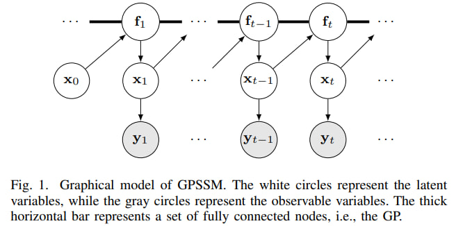
<p>The paper’s central idea is to put EnKF inside variational inference for GPSSMs. Variational inference normally introduces an approximate posterior distribution $q$ and optimizes an evidence lower bound, or <strong>ELBO</strong>. In many previous GPSSM methods, the distribution over hidden states is parameterized by many extra variables or by an inference network. That can be slow, unstable, and awkward for online learning.</p>

<p><img src="/images/blog/gauss_and_kalman/GPSSM.jpg" alt="Graphical model of GPSSM" /></p>

<p>EnVI changes the design:</p>

<div class="language-text highlighter-rouge"><div class="highlight"><pre class="highlight"><code>Noisy observations y_t
        |
        v
EnKF estimates hidden states x_t
        |
        v
Sparse GP learns transition f(x_t)
        |
        v
ELBO balances data fit + regularization
        |
        v
Updated model for filtering and forecasting
</code></pre></div></div>

<p>The approximate objective derived in the paper can be read as:</p>

\[\mathcal L \approx
\mathbb E_{q(u)}\left[\sum_{t=1}^T \log p(y_t \mid u, y_{1:t-1})\right]
- \mathrm{KL}(q(x_0)\|p(x_0))
- \mathrm{KL}(q(u)\|p(u)).\]

<p>The first term rewards predictions that explain the observations. The two KL terms act as regularizers: the initial state and the GP transition should not drift too far from their priors unless the data strongly supports it.</p>

<p>This is a nice objective because it is interpretable. The algorithm is not just fitting observations. It is also controlling model complexity and uncertainty.</p>

<h3 id="why-non-mean-field-matters">Why “non-mean-field” matters</h3>

<p>A mean-field approximation breaks dependencies between groups of variables. This often makes optimization easier, but in a dynamical model it can be too aggressive. The hidden states and transition function are deeply linked: changing the transition function changes the plausible hidden trajectory, and changing the hidden trajectory changes what transition function is learned.</p>

<p>EnVI keeps this relationship more naturally. The EnKF state estimates depend on the GP transition, and the GP is learned from those filtered states. This is why the paper calls the method non-mean-field: it does not pretend that the latent states and GP dynamics are independent.</p>

<h2 id="online-learning-oenvi">Online learning: OEnVI</h2>

<p>The online version, <strong>OEnVI</strong>, processes data one time step at a time. At each new observation it performs the same basic cycle:</p>

<ol>
  <li>sample or use the current GP surrogate;</li>
  <li>predict the ensemble forward;</li>
  <li>update the ensemble with the new observation;</li>
  <li>update model and variational parameters using the local objective.</li>
</ol>

<p>The online objective has the same spirit as the offline one:</p>

\[\mathcal L_t = \mathbb E_{q(u)}[\log p(y_t \mid u, y_{1:t-1})]
- \mathrm{KL}(q(u)\|p(u)).\]

<p>This matters because many systems do not arrive as a fixed dataset. Sensors, robots, vehicles, and monitoring systems stream data continuously. A method that requires the entire sequence at training time is less convenient there. OEnVI is designed to update as data arrives.</p>

<h2 id="what-tasks-does-this-combination-solve">What tasks does this combination solve?</h2>

<p>The GP-EnKF combination is useful for several related tasks:</p>

<table>
  <thead>
    <tr>
      <th>Task</th>
      <th>What the model does</th>
      <th>Why the combination helps</th>
    </tr>
  </thead>
  <tbody>
    <tr>
      <td>Filtering</td>
      <td>Estimate current hidden state from noisy observations</td>
      <td>EnKF corrects predictions using new measurements</td>
    </tr>
    <tr>
      <td>Dynamics learning</td>
      <td>Learn the unknown nonlinear transition function</td>
      <td>GP models flexible dynamics and reports uncertainty</td>
    </tr>
    <tr>
      <td>Forecasting</td>
      <td>Predict future observations and uncertainty</td>
      <td>The learned GP transition can be rolled forward</td>
    </tr>
    <tr>
      <td>Online inference</td>
      <td>Update the model as data streams in</td>
      <td>OEnVI avoids a heavy inference network trained on full sequences</td>
    </tr>
  </tbody>
</table>

<p>The key design choice is that EnKF handles the state-estimation part, while the GP handles the unknown-function part. Variational inference ties them together with a principled training objective.</p>

<h2 id="experimental-results-what-was-most-impressive">Experimental results: what was most impressive?</h2>

<p>The authors test the methods on synthetic and real datasets. The exact numbers are less important than the pattern: EnVI is usually more accurate, more robust, or faster to train than competing GPSSM and neural state-space methods.</p>

<h3 id="1-linear-gaussian-tracking-close-to-the-kalman-filter">1. Linear-Gaussian tracking: close to the Kalman filter</h3>

<p>The authors first use a setting where the classical Kalman filter is available as a strong reference: a linear-Gaussian car-tracking model. EnVI and OEnVI do not receive the true physical transition model, only noisy observations.</p>

<p>Even so, their state estimates are close to the Kalman filter baseline. The reported latent-state RMSE values are:</p>

<ul>
  <li>Kalman filter: <strong>0.5252</strong>;</li>
  <li>EnVI: <strong>0.6841</strong>;</li>
  <li>OEnVI: <strong>0.7784</strong>;</li>
  <li>raw observations versus latent states: <strong>0.9872</strong>.</li>
</ul>

<p>This experiment is a sanity check. If a learned GPSSM cannot do well on a linear-Gaussian system, it is hard to trust it on nonlinear ones. EnVI passes this check convincingly. OEnVI is less accurate at the beginning because it learns sequentially, but the paper reports that after more online data it improves substantially.</p>

<h3 id="2-kink-function-learning-nonlinear-dynamics-under-noise">2. Kink function: learning nonlinear dynamics under noise</h3>

<p>The kink function is a classic GPSSM test. It is a one-dimensional nonlinear transition that is simple enough to visualize but hard enough to expose bad uncertainty estimates.</p>

<p>Across three observation-noise levels, EnVI obtains the best transition-function fit among the compared methods. For example, at the lowest noise level, EnVI reports MSE <strong>0.0046</strong>, while AD-EnKF reports <strong>0.0285</strong>, VCDT <strong>0.2057</strong>, and vGPSSM <strong>1.0410</strong>. At high noise, EnVI still performs best: MSE <strong>0.5315</strong>, compared with <strong>1.3489</strong> for AD-EnKF, <strong>1.4035</strong> for VCDT, and <strong>1.9584</strong> for vGPSSM.</p>

<p>The visual result is also important: EnVI learns both the shape of the kink and a reasonable uncertainty band. The paper argues that AD-EnKF can become overconfident because it uses a deterministic neural transition model, while EnVI keeps uncertainty through the GP.</p>

<p>Another striking result is convergence. On the kink experiment, EnVI reaches good performance after roughly <strong>300 iterations</strong>, whereas vGPSSM and VCDT require many more iterations and more runtime. This supports the authors’ claim that removing a large inference network makes optimization easier.</p>

<h3 id="3-real-time-series-forecasting-strong-small-data-performance">3. Real time-series forecasting: strong small-data performance</h3>

<p>The paper also evaluates five public system-identification datasets: Actuator, Ball Beam, Drive, Dryer, and Gas Furnace. The model trains on the first half of each sequence and forecasts the second half. The reported metric is 50-step-ahead RMSE.</p>

<p>EnVI is best on four of the five datasets and competitive on the fifth. Its RMSEs are:</p>

<ul>
  <li>Actuator: <strong>0.657</strong>;</li>
  <li>Ball Beam: <strong>0.055</strong>;</li>
  <li>Drive: <strong>0.703</strong>;</li>
  <li>Dryer: <strong>0.125</strong>;</li>
  <li>Gas Furnace: <strong>1.388</strong>.</li>
</ul>

<p>The Drive dataset is the main exception: PRSSM reports <strong>0.647</strong>, better than EnVI’s <strong>0.703</strong>. But overall, the results are strong, especially because these datasets are relatively small. That is exactly the regime where GP-based models can be attractive compared with large neural models.</p>

<h3 id="4-online-nascar-dynamics-oenvi-wins-clearly">4. Online NASCAR dynamics: OEnVI wins clearly</h3>

<p>For online learning, the authors use a NASCAR-shaped latent trajectory and compare OEnVI with SVMC and VJF. The prediction RMSEs are:</p>

<ul>
  <li>OEnVI: <strong>1.8780</strong>;</li>
  <li>SVMC: <strong>4.6682</strong>;</li>
  <li>VJF: <strong>10.8499</strong>.</li>
</ul>

<p>This is one of the clearest experimental wins in the paper. OEnVI tracks and predicts the latent trajectory much better than the alternatives. The authors attribute this to the EnKF-based approximation of the latent-state distribution: it is structured enough to be stable, but flexible enough to work online.</p>

<h2 id="takeaways-and-limitations">Takeaways and limitations</h2>

<p>The paper is interesting because it does not simply replace everything with a neural network. It combines a probabilistic non-parametric model with a classical filtering algorithm, then trains the whole system with variational inference.</p>

<p>The main takeaways are:</p>

<ul>
  <li>GPSSMs are useful when the transition dynamics are unknown and nonlinear.</li>
  <li>EnKF provides a practical way to infer hidden states without a heavy inference network.</li>
  <li>The resulting ELBO has a clear interpretation: fit the observations, but regularize the initial state and transition function.</li>
  <li>OEnVI makes the method suitable for streaming data.</li>
  <li>The strongest empirical results are on nonlinear dynamics learning and online tracking.</li>
</ul>

<p>There are also natural limitations. EnKF relies on Gaussian-style updates, so it may struggle in strongly non-Gaussian settings where particle filters are more appropriate. The paper mainly uses a linear emission model, although EnKF can be extended to nonlinear emissions. Finally, the conclusion notes that time-varying dynamical systems remain an important direction for future work.</p>

<h2 id="useful-links-for-readers">Useful links for readers</h2>

<ul>
  <li>Original paper on arXiv: <a href="https://arxiv.org/abs/2312.05910">Ensemble Kalman Filtering Meets Gaussian Process SSM</a></li>
  <li>Authors’ GPSSM code repository: <a href="https://github.com/zhidilin/gpssmProj">zhidilin/gpssmProj</a></li>
  <li>A classic free book on Gaussian processes: <a href="https://gaussianprocess.org/gpml/">Gaussian Processes for Machine Learning</a></li>
  <li>Intuitive Kalman filtering book with Python code: <a href="https://rlabbe.github.io/Kalman-and-Bayesian-Filters-in-Python/">Kalman and Bayesian Filters in Python</a></li>
  <li>Practical GP library documentation: <a href="https://docs.gpytorch.ai/en/stable/examples/04_Variational_and_Approximate_GPs/index.html">GPyTorch variational and approximate GPs</a></li>
</ul>]]></content><author><name>Denis Rubtsov</name></author><category term="bmm" /><category term="gaussian processes" /><category term="kalman filter" /><summary type="html"><![CDATA[Why this paper matters]]></summary></entry><entry xml:lang="en"><title type="html">Proving the Lottery Ticket Hypothesis: Pruning is All You Need</title><link href="https://intsystems.github.io/materials/blog/lottery-ticket-pruning-is-all-you-need/" rel="alternate" type="text/html" title="Proving the Lottery Ticket Hypothesis: Pruning is All You Need" /><published>2026-05-14T00:00:00+00:00</published><updated>2026-05-14T00:00:00+00:00</updated><id>https://intsystems.github.io/materials/blog/lottery-ticket-pruning-is-all-you-need</id><content type="html" xml:base="https://intsystems.github.io/materials/blog/lottery-ticket-pruning-is-all-you-need/"><![CDATA[<h2 id="background-from-winning-tickets-to-a-stronger-claim">Background: from winning tickets to a stronger claim</h2>

<p>In 2018, Frankle and Carbin introduced the <a href="https://arxiv.org/abs/1803.03635">Lottery Ticket Hypothesis (LTH)</a>: a dense, randomly-initialized neural network contains a sparse subnetwork, a <em>winning ticket</em>, that, when trained in isolation from the original initialization, matches the accuracy of the full network. Empirically, such tickets can be 10 to 20 times smaller than the parent network.</p>

<p>LTH was a striking observation, but it left a theoretical gap. <em>Why</em> do such tickets exist? Are they an artifact of optimization, or a property of random networks themselves?</p>

<p>In <a href="http://proceedings.mlr.press/v119/malach20a/malach20a.pdf">Proving the Lottery Ticket Hypothesis: Pruning is All You Need</a> (ICML 2020), Malach, Yehudai, Shalev-Shwartz, and Shamir prove a much stronger version of LTH. Their result, sometimes called the Strong Lottery Ticket Hypothesis, says:</p>

<blockquote>
  <p>A sufficiently overparameterized randomly-initialized network contains a subnetwork that approximates any target function, with no training at all. Pruning alone is enough.</p>
</blockquote>

<p>This post walks through the statement, the proof idea, and what it does (and does not) say about deep learning in practice.</p>

<h2 id="the-setup">The setup</h2>

<p>Fix a target ReLU network $f^{\star}$ of depth $\ell$ and width $n$, with bounded weights $\lVert w \rVert \le 1$. We want to approximate $f^{\star}$ within error $\varepsilon$ on the unit ball.</p>

<p>The construction is:</p>

<ol>
  <li>Take a randomly-initialized ReLU network $G$ of depth $2\ell$ and width polynomial in $n, d, 1/\varepsilon, \log(1/\delta)$.</li>
  <li>Do not train it. Instead, select a binary mask $M$ over its weights.</li>
  <li>Show that $M \odot G$ approximates $f^{\star}$ uniformly with high probability $1 - \delta$.</li>
</ol>

<p>The notable points: depth only doubles, width is polynomial, weights are never modified; they are only kept or zeroed out.</p>

<h2 id="the-main-theorem-informal">The main theorem (informal)</h2>

<p>Let $f^{\star}$ be any ReLU network of depth $\ell$, width $n$, and bounded weights. For any $\varepsilon, \delta &gt; 0$, a random ReLU network of depth $2\ell$ and width polynomial in $n, \ell, d, 1/\varepsilon, \log(1/\delta)$ contains, with probability at least $1 - \delta$, a subnetwork that uniformly $\varepsilon$-approximates $f^{\star}$ on the unit ball. The number of active (non-pruned) weights in the subnetwork is $O(dn + n^2 \ell)$, the same order as the parameter count of $f^{\star}$.</p>

<p>In other words: expressivity of pruning a random net equals expressivity of training a net of the same target size, up to polynomial overhead in width.</p>

<p>The paper focuses on weight-pruning, where individual weights can be zeroed independently. A separate result (Theorem 3.2) shows that the strictly weaker model of <em>neuron-pruning</em>, in which only entire neurons can be removed, is equivalent to random features and therefore cannot achieve the same expressive power. This post discusses only the weight-pruning result.</p>

<h2 id="the-proof-idea-approximate-each-weight-by-two-random-relus">The proof idea: approximate each weight by two random ReLUs</h2>

<p>The core trick is local: replace each scalar weight $w \in [-1, 1]$ in the target network by a tiny gadget built from random neurons in the random network.</p>

<h3 id="step-1-a-single-weight-from-two-relus">Step 1: a single weight from two ReLUs</h3>

<p>The building block is the identity
\(a = \sigma(a) - \sigma(-a)\)
where $\sigma$ is the ReLU. Applied coordinate-wise, this lets us write any signed product $w \cdot x$ as
\(w \cdot x = \sigma(w \cdot x) - \sigma(-w \cdot x)\)
so two ReLU units with input weights $+w$ and $-w$ (and output signs $+1$ and $-1$) reproduce the linear function $x \mapsto w \cdot x$ exactly.</p>

<p>In the random network we do not have $\pm w$ available, but we have a <em>pool</em> of many random scalars. The pool is wide enough that, with high probability, it contains a pair of values close to $+w$ and $-w$ within accuracy $\varepsilon_0$. Pruning everything else leaves a two-neuron gadget that approximates $w \cdot x$.</p>

<h3 id="step-2-pick-by-pruning">Step 2: pick by pruning</h3>

<p>The random network has many neurons in each layer. For each target weight, the construction prunes away all neurons in the pool except the two chosen ones approximating $+w$ and $-w$. Combined with the next layer’s $+1/-1$ outgoing weights (also obtained by pruning), the remaining two neurons implement an approximation of $w \cdot x$.</p>

<h3 id="step-3-error-accumulation">Step 3: error accumulation</h3>

<p>Each weight is approximated to error $\varepsilon_0$. The approximation errors propagate through $\ell$ layers, and by Lipschitz arguments on bounded-weight networks, the total error is $\mathrm{poly}(\ell, n) \cdot \varepsilon_0$. Choosing $\varepsilon_0$ small enough gives uniform $\varepsilon$-approximation of $f^{\star}$.</p>

<h3 id="why-depth-doubles">Why depth doubles</h3>

<p>Each target layer is implemented by two layers of the random network: one for the pool of random scalars feeding the ReLU pair, one for combining them with $\pm 1$ outgoing weights. Hence depth $2\ell$.</p>

<h3 id="why-width-is-polynomial">Why width is polynomial</h3>

<p>For each target weight, the pool has to be large enough that two random scalars fall within $\varepsilon_0$ of any target value in $[-1, 1]$. A covering argument on $[-1, 1]$ shows this requires $\widetilde{O}(1/\varepsilon_0^{2})$ random samples per weight, and a union bound over all $n^2 \ell$ weights yields a polynomial width.</p>

<h2 id="what-this-changes-about-how-we-think-about-pruning">What this changes about how we think about pruning</h2>

<p>Pruning is at least as expressive as training. Up to polynomial overhead in width, anything a trained network of size $n$ can represent can also be represented by pruning a random network of size $\mathrm{poly}(n)$. Empirical pruning algorithms are searching over a hypothesis class that is, in principle, rich enough.</p>

<p>The winning ticket is universal. The same random network contains tickets for <em>every</em> target; the choice of mask depends on $f^{\star}$, but the random weights do not.</p>

<p>It partially explains why pruning works so well after training. If subnetworks of the <em>initial</em> random network can already approximate good functions, it is not surprising that subnetworks of a <em>trained</em> network can match its accuracy.</p>

<h2 id="important-caveats">Important caveats</h2>

<p>The result is an existence theorem, and several gaps remain between the proof and practice:</p>

<ol>
  <li>No algorithm. The proof tells us a good mask exists but not how to find it. Finding the optimal subnetwork is, in the worst case, computationally hard. Practical methods (magnitude pruning, edge-popup, lottery-ticket rewinding) are heuristics.</li>
  <li>Polynomial overparameterization. The width bound is polynomial in the target size, the input dimension, and $1/\varepsilon$. The exponents in the original proof are not tight, and for realistic $n$ the implied constants are large.</li>
  <li>Bounded weights and bounded inputs. The construction requires weight and input norms to be bounded, which is the standard but non-trivial assumption.</li>
  <li>No generalization claim. The theorem is about <em>approximation</em>, not learning. It does not say that a pruned random network will generalize from finite data the way a trained one does.</li>
</ol>

<p>Follow-up work has tightened these bounds. <a href="https://arxiv.org/abs/2006.07990">Pensia et al. (2020)</a> showed that the width overhead can be reduced to <em>logarithmic</em> in $1/\varepsilon$, bringing the strong LTH much closer to a tight statement.</p>

<h2 id="takeaways">Takeaways</h2>

<p>Frankle and Carbin’s empirical LTH said: train, then prune to find a winning ticket. Malach et al.’s strong LTH says: you don’t even need to train. The winning ticket is already there in the random initialization, waiting to be uncovered by a mask.</p>

<p>The proof is a clean, constructive argument: approximate every target weight by a difference of two random ReLUs, prune away the rest, and propagate the error through the layers.</p>

<p>The result is theoretical, and finding the mask remains the hard part, but it cleanly separates expressivity (which pruning a random net already has) from the algorithmic question of how to find a good subnetwork.</p>

<p>Pruning, viewed this way, is not a compression heuristic applied after the fact. It is a legitimate alternative form of “training”, and the strong LTH is the formal statement that it is, in principle, sufficient.</p>

<h2 id="references">References</h2>

<ol>
  <li>Malach, E., Yehudai, G., Shalev-Shwartz, S., &amp; Shamir, O. (2020). <em>Proving the Lottery Ticket Hypothesis: Pruning is All You Need</em>. ICML 2020. <a href="http://proceedings.mlr.press/v119/malach20a/malach20a.pdf">PDF</a></li>
  <li>Frankle, J., &amp; Carbin, M. (2018). <em>The Lottery Ticket Hypothesis: Finding Sparse, Trainable Neural Networks</em>. arXiv preprint, later published at ICLR 2019. <a href="https://arxiv.org/abs/1803.03635">arXiv:1803.03635</a></li>
  <li>Pensia, A., Rajput, S., Nagle, A., Vishwakarma, H., &amp; Papailiopoulos, D. (2020). <em>Optimal Lottery Tickets via Subset Sum: Logarithmic Over-Parameterization is Sufficient</em>. NeurIPS 2020. <a href="https://arxiv.org/abs/2006.07990">arXiv:2006.07990</a></li>
  <li>Ramanujan, V., Wortsman, M., Kembhavi, A., Farhadi, A., &amp; Rastegari, M. (2020). <em>What’s Hidden in a Randomly Weighted Neural Network?</em> CVPR 2020. <a href="https://arxiv.org/abs/1911.13299">arXiv:1911.13299</a></li>
</ol>]]></content><author><name>Gleb Karpeev</name></author><category term="bmm" /><category term="Deep Learning" /><category term="pruning" /><category term="lottery ticket hypothesis" /><summary type="html"><![CDATA[Background: from winning tickets to a stronger claim]]></summary></entry><entry xml:lang="en"><title type="html">Gradient-based Hyperparameter Optimization Over Long Horizons</title><link href="https://intsystems.github.io/materials/blog/fds/" rel="alternate" type="text/html" title="Gradient-based Hyperparameter Optimization Over Long Horizons" /><published>2026-03-02T00:00:00+00:00</published><updated>2026-03-02T00:00:00+00:00</updated><id>https://intsystems.github.io/materials/blog/fds</id><content type="html" xml:base="https://intsystems.github.io/materials/blog/fds/"><![CDATA[<p><strong>Based on the 2021 NeurIPS conference paper by Paul Micaelli and Amos Storkey</strong></p>

<p><em>If you find this topic interesting, please check out the <a href="https://proceedings.neurips.cc/paper/2021/file/596dedf4498e258e4bdc9fd70df9a859-Paper.pdf">original paper</a></em>!</p>

<h2 id="introduction">Introduction</h2>

<p><strong>Hyperparameter optimization</strong> <strong>(HPO)</strong> is a rapidly developing direction in the field of machine learning and optimization. It considers the automatic optimization of <em>hyperparameters</em> (<em>outer optimization</em>), for example, optimizer parameters like learning rate or weight decay, on top of the optimization of model parameters (<em>inner optimization</em>). In this post we will be looking at one of the <strong>gradient-based</strong> HPO methods, i.e. methods that rely on the differentiability of certain hyperparameters for their optimization. Such methods are able to utilize gradient information rather than relying on trial-and-error and thus have earned a widespread popularity in the context of few-shot meta-learning. However, at the time these methods were broadly impractical for long-horizon tasks (tasks with many gradient steps in each training cycle). But why?</p>
<h3 id="problems-of-previous-methods">Problems of previous methods</h3>

<p>Typically previous gradient-based HPO methods relied on <a href="https://www.researchgate.net/profile/Paul-Werbos/publication/2984354_Backpropagation_through_time_what_it_does_and_how_to_do_it/links/55ef061c08aef559dc44b02d/Backpropagation-through-time-what-it-does-and-how-to-do-it.pdf">backpropagation through time (BPTT)</a>. Unfortunately, this procedure is extremely expensive both in time and memory, and because of that most previously proposed methods were limited to toy models and datasets. Moreover, long optimization horizons cause hypergradient degradation (i.e. exploding or vanishing hypergradients).</p>

<p>One type of methods that allows to alleviate both these problems is <strong>greedy methods</strong>. This refers to finding the best hyperparameters locally rather than globally, typically by splitting the inner optimization problem into smaller chunks (often just one batch) and solving for hyperparameters over these smaller horizons instead. However, such methods <a href="https://arxiv.org/pdf/1803.02021">had been found to introduce bias</a> in the HPO process and thus solve for the wrong objective. The paper we’ll discuss focuses on extending gradient-based methods to the non-greedy setting.</p>

<p>Many previously existing methods were not gradient-based. The most popular ones at the time were black-box methods like <a href="https://www.jmlr.org/papers/volume18/16-558/16-558.pdf">Hyperband</a> and its combination with Bayesian optimization called <a href="https://proceedings.mlr.press/v80/falkner18a/falkner18a.pdf">BOHB</a>. These methods rely on trial-and-error, and, as we will see later on, reach optima way slower than gradient-based alternatives such as the one we’ll look at in this post.</p>

<h2 id="method-forward-mode-differentiation-with-hyperparameter-sharing">Method: Forward-Mode Differentiation with Hyperparameter Sharing</h2>

<p>In their paper, Micaelli and Storkey introduce <strong>Forward-mode Differentiation with hyperparameter Sharing (FDS)</strong>, which proposes the following solutions to the aforementioned problems:</p>

<p>1) The use of <strong>gradients</strong> for optimization allows to reach global optima faster than by trial-and-error;
2) <strong>Forward-mode differentiation</strong> solves the memory efficiency problem, boasting a memory cost constant with optimization horizon size;
3) <strong>Hyperparameter sharing</strong> tackles gradient degradation by averaging hyperparameters over time.</p>

<p>Let’s see how this method works step by step.</p>

<h3 id="problem-statement">Problem statement</h3>

<p>Let’s denote:</p>

<ul>
  <li>$\boldsymbol{\theta}$ - the weights of the given neural network model.</li>
  <li>$\mathcal{L}$ - the loss function to be optimized.</li>
  <li>$\mathcal{D}$ - a dataset with train split $\mathcal{D}_\text{train}$ and validation split $\mathcal{D}_\text{val}$.</li>
  <li>$\Phi$ - a gradient-based optimizer for $\boldsymbol{\theta}$.</li>
  <li>$\boldsymbol{\lambda}_{[t]}$ - the set of hyperparameters that $\Phi$ uses for the optimization step $t$ (to get $\boldsymbol{\theta}_{t}$ from $\boldsymbol{\theta}_{t-1}$). Note that this implies that $\boldsymbol{\theta}_t = \boldsymbol{\theta}_t(\boldsymbol{\lambda}_{[1:t]})$.</li>
  <li>$\boldsymbol{\lambda} = \boldsymbol{\lambda}_{[1:T]}$ - the full set of hyperparameters used by $\Phi$ for optimization.</li>
  <li>$T$ - the number of optimization steps $\Phi$ takes.</li>
</ul>

<p>Our task is to find the optimal set of hyperparameters $\boldsymbol{\lambda}^*$ such that the result at time $T$ of the gradient process optimizing the train loss $\mathcal{L}_\text{train}$ also minimizes the generalization loss $\mathcal{L}_\text{val}$ on the validation set $\mathcal{D}_\text{val}$:</p>

\[\boldsymbol{\lambda}^* = \arg\min_\boldsymbol{\lambda} \mathcal{L}_\text{val}(\boldsymbol{\theta}_T, \mathcal{D}_\text{val}), 
\quad \text{subject to } \boldsymbol{\theta}_{t+1} = \Phi(\mathcal{L}_\text{train}(\boldsymbol{\theta}_{t}(\boldsymbol{\lambda}_{[1:t]}), \mathcal{D}_\text{train}), \boldsymbol{\lambda}_{[t+1]}).\]

<p>Here, the inner optimization loop, optimizing $\boldsymbol{\theta}$, expresses a constraint on the outer loop, optimizing $\boldsymbol{\lambda}$.</p>

<p>Let $H$ be the horizon, which corresponds to the number of optimization steps taken in the inner loop before a step is taken in the outer loop (optimizing the hyperparameters). If we solve this problem non-greedily, we have $T=H$. This means that non-greedy methods, like FDS, only update $\boldsymbol{\lambda}_{[t]}$ at time $T$. If we, on the other hand, consider a greedy approach, we get $H\ll T$. For example, <a href="https://arxiv.org/pdf/1703.04782">Hypergradient Descent (HD)</a>, a standard gradient-based HPO method, uses $H=1$.</p>

<p>The memory cost of BPTT, the go-to method for solving the optimization problem above, is $\mathcal{O}(DH)$, where $D$ is the number of weights. This estimate scales unfavorably when the optimization horizon is long. Greedy approaches help mitigate the memory scaling problem by minimizing $H$, yet bring about problems with minimizing the real objective. Forward-mode differentiation aims to improve the memory cost even in the non-greedy case.</p>

<h3 id="forward-mode-differentiation">Forward-mode differentiation</h3>

<p>Let’s consider the general case of using one hyperparameter $\boldsymbol{\lambda}_t$ per step. First, we use the chain rule, knowing that $\partial\mathcal{L}_\text{val}/\partial\boldsymbol{\lambda} = 0$ since the loss function doesn’t directly depend on the hyperparameters:</p>

\[\frac{d\mathcal{L}_\text{val}}{d\boldsymbol{\lambda}} = \frac{\partial\mathcal{L}_\text{val}}{\partial\boldsymbol{\theta_{T}}} \frac{d\boldsymbol{\theta_{T}}}{d\boldsymbol{\lambda}}.\]

<p>The first can be calculated as usual through backpropagation. The second term can be calculated recursively, again using the chain rule:</p>

\[\frac{d\boldsymbol{\theta_t}}{d\boldsymbol{\lambda}} = \left.\frac{\partial\boldsymbol{\theta_t}}{\partial\boldsymbol{\theta_{t-1}}}\right|_\boldsymbol{\lambda} \frac{d\boldsymbol{\theta_{t-1}}}{d\boldsymbol{\lambda}} + \left.\frac{\partial\boldsymbol{\theta_t}}{\partial\boldsymbol{\lambda}}\right|_\boldsymbol{\theta_{t-1}}\]

<p>We can write this as</p>

\[\mathbf{Z}_t = \mathbf{A}_t \mathbf{Z}_{t-1} + \mathbf{B}_t.\]

<p>The expressions for $\mathbf{A}_t$ and $\mathbf{B}_t$ depend on the specific hyperparameters used. The authors give an example for SGD with momentum with learning rate $α_t$, momentum $β_t$, weight decay $ξ_t$ and velocity $\mathbf{\nu}_t=\beta_t\mathbf{\nu}_{t-1}+\partial\mathcal{L}_\text{train}/\partial\boldsymbol{\theta}_{t-1})+\xi_t\boldsymbol{\theta}_{t-1}$:</p>

\[\left\{
\begin{array}{ll}
\mathbf{A}_t^\alpha = \mathbf{1} - \alpha_t\left(\frac{\partial^2\mathcal{L}_{\mathrm{train}}}{\partial\theta_{t - 1}^2} +\xi_t\mathbf{1}\right)\\[10pt]
\mathbf{B}_t^\alpha = -\beta_t\alpha_t\mathbf{C}_{t - 1}^\alpha -\delta_t^\otimes \left(\beta_t\boldsymbol{\nu}_{t - 1} + \frac{\partial\mathcal{L}_{\mathrm{train}}}{\partial\theta_{t - 1}} +\xi_t\theta_{t - 1}\right)\\[10pt]
\mathbf{C}_t^\alpha = \beta_t\mathbf{C}_{t - 1}^\alpha +\left(\xi_t\mathbf{1} + \frac{\partial^2\mathcal{L}_{\mathrm{train}}}{\partial\theta_{t - 1}^2}\right)\mathbf{Z}_{t - 1}^\alpha
\end{array}
\right.\]

<p>Here, a further recursive term $\mathbf{C}_t = (\partial\mathbf{v}_t/\partial\boldsymbol{\lambda})$ must be considered to get exact hypergradients.</p>

<p>Forward-mode differentiation scales in memory as $\mathcal{O}(DN)$, where $N$ is the number of learnable hyperparameters. The additional scaling by $N$ is a limitation in case we learn one hyperparameter per inner step ($N=T$). However, we can conveniently allow for smaller values of $N$ using hyperparameter sharing.</p>

<h3 id="hyperparameter-sharing">Hyperparameter sharing</h3>

<p>As we noticed earlier, one problem of non-greedy HPO methods is gradient degradation. Specifically, small changes in initial parameters like weight initialization and minibatch ordering can drastically affect hypergradients, introducing large fluctuations. Ideally, hyperparameters should be agnostic to such factors, so we would like to average out their effect on hypergradients. However, the most obvious way of doing that, <em>ensemble averaging</em>, has very high computational and memory cost. FDS utilizes a different strategy - <strong>time averaging</strong>.</p>

<p>The idea of time averaging is to average out hypergradients across the inner training loop rather than the outer loop. Specifically, in FDS we average out hypergradients from $W$ neighboring time steps in the inner loop, which is, in fact, equivalent to sharing one hyperparameter over all these steps. This helps reduce gradient degradation, but introduces a bias, since in general ensemble averaging and time averaging aren’t equivalent. Nevertheless, the authors manage to prove that the hypergradient error $\text{MSE}_W$ with sharing (specifically, the mean variance of the hypergradient, given that it can be approximated with a Gaussian) has the following upper bound:</p>

\[\text{MSE}_W &lt; \frac{(1+c(W - 1))}{W}\text{MSE}_1 + L^2\frac{W^2 - 1}{12},\]

<p>where $c$ is the maximum absolute correlation between hypergradients, $L$ is the Lipschitz constant for the network, and $\text{MSE}_1$ is the hypergradient error without hyperparameter sharing. In fact, this entails that for sufficiently small $c$ and $L$, we actually end up with $\text{MSE}_W &lt; \text{MSE}_1$ for some positive $W$.</p>

<h2 id="experiments">Experiments</h2>

<p>The paper’s authors conducted several experiments to test FDS on long-horizon tasks in comparison with state-of-the-art methods at the time to test whether the proposed method shows its main benefits in practice.</p>

<h3 id="the-effect-of-hyperparameter-sharing-on-hypergradient-noise">The effect of hyperparameter sharing on hypergradient noise</h3>

<p><img src="/images/blog/fds/figure2.png" alt="" />
<em><strong>Figure 1:</strong> Hypergradients on SVHN for 100 seeds in the non-greedy (left) and greedy (middle) setting. The mean squared error is also shown (right).</em></p>
<p>The first experiment tested how well hyperparameter sharing dealt with hypergradient noise and how it affected the hypergradient error, training the learning rate for LeNet on the SVHN dataset. The method did, in fact, outperform the greedy setting, significantly reducing noise for many values of $W$. Interestingly, the mean squared error of the gradient has also significantly reduced, showing the best result for $W=50$.</p>

<h3 id="the-effect-of-hyperparameter-sharing-on-hpo">The effect of hyperparameter sharing on HPO</h3>

<p><img src="/images/blog/fds/figure3.png" alt="" />
<em><strong>Figure 2:</strong> The learning rate schedule learned on MNIST and SVHN using LeNet.</em></p>
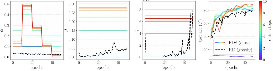
<p>The next two experiments analyze how hyperparameter sharing affects performance of HPO on various real datasets. In the Figure 2, we can see the results of training the learning rate for LeNet on MNIST and SVHN. Despite LeNet being a relatively small architecture, making non-greedy HPO a viable option, both greedy and non-greedy HPO fail to find reasonable learning rates for training on SVHN, probably due to hypergradient variance. On the other hand, FDS stabilizes non-greedy hypergradients and allows to find learning rates that even outperform reasonable off-the-shelf schedules (cosine annealing in this case).</p>

<p><img src="/images/blog/fds/figure4.png" alt="" />
<em><strong>Figure 3:</strong> FDS applied to SGD with momentum to learn the learning rate schedule $\alpha$, momentum $\beta$ and weight decay $\xi$.</em></p>
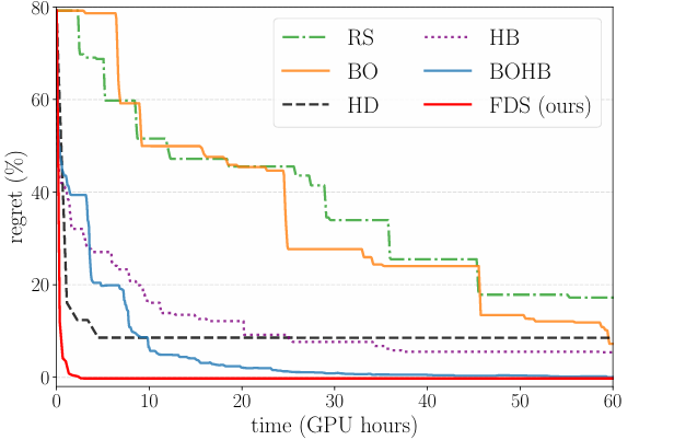
<p>Figure 3 shows the results of an experiment with a larger model, WideResNet-16-1, on the CIFAR-10 dataset. Due to the size of the model, non-greedy HPO without hyperparameter sharing becomes too computationally expensive, so the authors only compared FDS with a greedy method, Hypergradient Descent (HD). This experiment shows that in just 10 outer steps, FDS manages to converge to noticeably more reasonable values of the hyperparameters than HD, resulting in better test performance while still being a viable option in this setting.</p>

<h3 id="fds-vs-other-hpo-methods">FDS vs. other HPO methods</h3>

<p><img src="/images/blog/fds/figure1.png" alt="" />
<em><strong>Figure 4:</strong> Performance of the most popular HPO methods on CIFAR-10 for a WideResNet-16.</em></p>
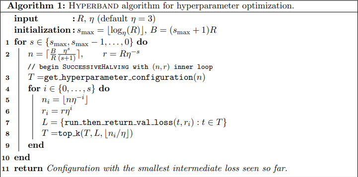
<p>The last experiment aims to demonstrate why FDS is such a valuable method compared to others used before it. We can see that non-greedy methods like random search (RS), Bayesian optimization (BO), Hyperband (HB) and the combination of the latter two (BOHB), while solving for global optima, rely on trial-and-error, which makes them very slow. On the other hand, greedy methods like Hypergradient Descent (HD) are faster but solve for local optima. FDS manages to take the best of both worlds, outperforming even the next best method while converging 20 times faster.</p>

<h2 id="conclusion">Conclusion</h2>

<p>FDS has been proven to be a well-balanced alternative to the state-of-the-art methods at the time, and its notable performance still makes it a strong baseline to this day. While the field of HPO has since then developed quite significantly, FDS is still worth considering in various applications, given its strengths.</p>

<p><strong>Main strengths of FDS:</strong></p>
<ul>
  <li><strong>Hypergradient noise reduction</strong>: hyperparameter sharing allows to combat gradient degradation, reducing the hypergradient error for optimal configurations of $W$ (for many purposes $W=50$ proved to be quite optimal).</li>
  <li><strong>Accuracy</strong>: offers better accuracy without trade-offs in comparison to greedy methods.</li>
  <li><strong>Convergence speed:</strong> converges much faster than trial-and-error methods.</li>
</ul>

<p><strong>Limitations:</strong></p>
<ul>
  <li><strong>Requires differentiable hyperparameters:</strong> to use FDS with discrete hyperparameters, you will need to perform relaxation.</li>
  <li><strong>Memory requirements scale linearly</strong> with the amount of hyperparameters. For example, a 12 GB GPU can train up to ~$10^3$ hyperparameters.</li>
  <li><strong>Recurrent formulas are parameter-specific:</strong> each type of hyperparameter will require the derivation of its own expressions for matrices $\mathbf{A}_t$ and $\mathbf{B}_t$.</li>
</ul>]]></content><author><name>Fedor Sobolevsky</name></author><category term="Hyperparameter optimization" /><category term="BMM" /><summary type="html"><![CDATA[Based on the 2021 NeurIPS conference paper by Paul Micaelli and Amos Storkey]]></summary></entry><entry xml:lang="en"><title type="html">Hyperband: Accelerating Hyperparameter Optimization via Adaptive Resource Allocation</title><link href="https://intsystems.github.io/materials/blog/hyperband/" rel="alternate" type="text/html" title="Hyperband: Accelerating Hyperparameter Optimization via Adaptive Resource Allocation" /><published>2026-02-17T00:00:00+00:00</published><updated>2026-02-17T00:00:00+00:00</updated><id>https://intsystems.github.io/materials/blog/hyperband</id><content type="html" xml:base="https://intsystems.github.io/materials/blog/hyperband/"><![CDATA[<h2 id="some-background">Some background</h2>

<p>Hyperparameter Optimization (HPO) remains one of the most resource-intensive bottlenecks in the machine learning pipeline. While the community has largely moved past Grid Search, the standard alternatives — Random Search and Bayesian Optimization — still suffer from a fundamental inefficiency: they treat the training process as a “black box” that must be run to completion.</p>

<p>In 2018, Lisha Li and researchers from Carnegie Mellon, Google, and the University of Washington published the paper <a href="https://arxiv.org/abs/1603.06560"><strong>“Hyperband: A Novel Bandit-Based Approach to Hyperparameter Optimization.”</strong></a> They proposed a paradigm shift: instead of trying to <em>intelligently select</em> configurations (as Bayesian methods do), we should focus on efficiently evaluating them using adaptive resource allocation.</p>

<p>In this post, we will deconstruct the Hyperband algorithm, the theoretical problem it solves, and why it often outperforms Bayesian methods.</p>

<h2 id="the-core-problem-the-n-vs-bn-tradeoff">The Core Problem: The “n vs. B/n” Tradeoff</h2>

<p>The central challenge in random search-based HPO is resource allocation. Suppose you have a total finite budget $B$ (e.g., total GPU hours). You need to decide how many unique hyperparameter configurations $n$ to evaluate.</p>

<p>This creates a fundamental tradeoff:</p>

<ol>
  <li><strong>Maximize $n$ (Width):</strong> You sample many configurations to cover the search space, but each gets a very small average budget ($B/n$).
    <ul>
      <li><em>Risk:</em> You might stop a promising configuration too early (“false negative”).</li>
    </ul>
  </li>
  <li><strong>Minimize $n$ (Depth):</strong> You sample few configurations, but train them to convergence.
    <ul>
      <li><em>Risk:</em> You train a poor configuration for too long, wasting resources that could have been used to explore other areas of the search space.</li>
    </ul>
  </li>
</ol>

<p>For a fixed budget, it is impossible to know which strategy — width or depth — will yield the best model. Hyperband was designed specifically to solve this dilemma.</p>

<h2 id="the-building-block-successive-halving">The Building Block: Successive Halving</h2>

<p>To understand Hyperband, one must first understand its subroutine: <strong>Successive Halving (SH)</strong>. Originally proposed for multi-armed bandit problems, SH operates like a tournament:</p>

<ol>
  <li><strong>Initialize:</strong> Start with <strong>$n$</strong> randomly sampled configurations.</li>
  <li><strong>Evaluate:</strong> Allocate a small budget <strong>$r$</strong> (e.g., 1 epoch) to all configurations.</li>
  <li><strong>Select:</strong> Rank them by validation loss and discard the worst half.</li>
  <li><strong>Promote:</strong> The surviving configurations are promoted to the next round with a larger budget.</li>
  <li><strong>Repeat:</strong> Continue until one configuration remains.</li>
</ol>

<p>While SH is efficient, it still requires the user to choose $n$. Given some finite budget $B$, if $n$ is too large, the initial budget $r$ might be too small to distinguish good models from bad ones. If $n$ is too small, SH behaves like standard Random Search.</p>

<h2 id="the-hyperband-algorithm">The Hyperband Algorithm</h2>

<p>Hyperband acts as a “wrapper” or an outer loop around Successive Halving. Instead of forcing the user to guess the optimal $n$, Hyperband iterates through different feasible values of $n$ for a fixed total budget.</p>

<p>It divides the total budget into several <strong>“brackets”</strong> (instances of Successive Halving):</p>

<ul>
  <li><strong>Most Aggressive Bracket ($s = s_{max}$):</strong> Starts with the maximum possible number of configurations ($n_{max}$) with the minimum resource per config. This is designed to identify “fast learners” quickly.</li>
  <li><strong>Intermediate Brackets:</strong> Gradually decrease $n$ and increase the initial resource $r$.</li>
  <li><strong>Most Conservative Bracket ($s = 0$):</strong> Starts with a small number of configurations but allocates the maximum resource immediately. This is essentially equivalent to standard Random Search (exploration) or simply training to convergence (exploitation).</li>
</ul>

<h3 id="algorithm-inputs">Algorithm Inputs</h3>

<p>Hyperband is notably easy to configure, requiring only two inputs:</p>

<ol>
  <li><strong>$R$</strong>: The maximum amount of resource that can be allocated to a single configuration (e.g., 100 epochs, or the full dataset size).</li>
  <li><strong>$\eta$</strong>: The proportion of configurations discarded in each round of Successive Halving.</li>
</ol>

<p><img src="/images/blog/hyperband/algorithm.png" alt="Pseudocode of the Hyperband algorithm showing the outer loop for brackets and inner loop for Successive Halving." /></p>

<p>By iterating through these brackets, Hyperband performs a geometric search over the trade-off between “number of configurations” and “resource per configuration.”</p>

<h2 id="theoretical-framework-the-infinite-armed-bandit">Theoretical Framework: The Infinite-Armed Bandit</h2>

<p>The authors frame HPO as a non-stochastic infinite-armed bandit problem.</p>

<ul>
  <li><strong>Infinite-armed:</strong> The hyperparameters are drawn from a continuous probability distribution.</li>
  <li><strong>Non-stochastic:</strong> The algorithm does not make strong assumptions about the convergence curves of the loss functions.</li>
</ul>

<p>This theoretical grounding is significant because it contrasts with Bayesian Optimization (BO). BO relies on fitting a probabilistic model to the function $f(x)$. In high-dimensional spaces, fitting this model becomes computationally expensive and often inaccurate. Hyperband avoids this complexity entirely by relying on principled random sampling and aggressive early stopping.</p>

<h2 id="empirical-results">Empirical Results</h2>

<p>The paper presents extensive evaluation comparing Hyperband against Random Search, SMAC, TPE, and Spearmint (popular Bayesian optimization frameworks) on several benchmarks.</p>

<h3 id="1-deep-learning-iterations-as-resource">1. Deep Learning (Iterations as Resource)</h3>

<p>In this experiment, the authors tuned Convolutional Neural Networks (CNNs) on datasets like CIFAR-10 and SVHN. The resource budget was defined as the number of training iterations (epochs).</p>

<p><img src="/images/blog/hyperband/image-deeplearning.png" alt="Average test error across 10 trials on CIFAR-10." /></p>

<p><em>Average test error across 10 trials. Label “SMAC (early)” corresponds to SMAC with the early-stopping criterion and label “bracket s = 4” corresponds to repeating the most exploratory bracket of Hyperband. <strong>Result: Hyperband found high-quality configurations 5× to 30× faster than Bayesian methods.</strong></em></p>

<h3 id="2-kernel-methods-data-subsampling-as-resource">2. Kernel Methods (Data Subsampling as Resource)</h3>

<p>Here, the task was Kernel Least Squares classification. The resource was the size of the dataset subsample.</p>

<p><img src="/images/blog/hyperband/image-kernel.png" alt="Comparison of Hyperband and other methods on Kernel Least Squares classification tasks." /></p>

<p><em>On left: Average test error of the best kernel regularized least square classification model found by each searcher on CIFAR-10. On right: Average test error of the best random features model. <strong>Result: Hyperband achieved a massive 70× speedup over Random Search.</strong></em></p>

<h3 id="3-generalization-117-openml-datasets">3. Generalization (117 OpenML Datasets)</h3>

<p>To test robustness, Hyperband was evaluated on a large-scale automated machine learning task involving 117 real-world datasets from OpenML.</p>

<p><img src="/images/blog/hyperband/image-openmldatasets.png" alt="Average rank across all data sets for each searcher." /></p>

<p><em>Average rank across all data sets for each searcher. For each data set, the searchers are ranked according to the average validation/test error across 20 trials.</em></p>

<ul>
  <li><strong>Avoiding Overfitting:</strong> A key finding was that Bayesian optimization methods often “overfit” the validation set — they found configurations that looked good during search but performed worse on the test set. Hyperband, being closer to Random Search in its sampling strategy, showed better generalization.</li>
  <li><strong>Cost vs. Benefit:</strong> On a subset of 21 datasets where subsampling yielded meaningful computational speedups, Hyperband was the clear winner. However, on very small datasets where training takes seconds, the overhead of Hyperband made it less effective than simple Random Search.</li>
</ul>

<h2 id="conclusion">Conclusion</h2>

<p>The Hyperband paper provides a compelling argument that in the era of expensive model training, adaptive resource allocation is more critical than adaptive configuration selection.</p>

<p><strong>Key Practical Takeaways:</strong></p>

<ol>
  <li><strong>Efficiency:</strong> For problems where partial training (e.g., few epochs) correlates with final performance, Hyperband is superior to standard Random Search and often beats Bayesian Optimization.</li>
  <li><strong>Simplicity:</strong> It requires minimal tuning compared to the complex kernels and acquisition functions of Gaussian Processes.</li>
  <li><strong>Parallelism:</strong> The algorithm is easily parallelizable, making it ideal for modern distributed computing clusters.</li>
</ol>

<p>Today, Hyperband has become an industry standard, available in major HPO frameworks such as <strong>Ray Tune</strong>, <strong>Optuna</strong>, and <strong>Scikit-learn</strong> (<code class="language-plaintext highlighter-rouge">HalvingRandomSearchCV</code>). For anyone dealing with computationally expensive model tuning, it is a valuable tool in the machine learning toolkit.</p>]]></content><author><name>Dmitrii Vasilenko</name></author><category term="bmm" /><category term="hyperparameter optimization" /><category term="Deep Learning" /><summary type="html"><![CDATA[Some background]]></summary></entry><entry xml:lang="en"><title type="html">Understanding Invariance via Feedforward Inversion of Discriminatively Trained Classifiers</title><link href="https://intsystems.github.io/materials/blog/feedforward-classifier-inversion/" rel="alternate" type="text/html" title="Understanding Invariance via Feedforward Inversion of Discriminatively Trained Classifiers" /><published>2025-12-15T00:00:00+00:00</published><updated>2025-12-15T00:00:00+00:00</updated><id>https://intsystems.github.io/materials/blog/feedforward-classifier-inversion</id><content type="html" xml:base="https://intsystems.github.io/materials/blog/feedforward-classifier-inversion/"><![CDATA[<h2 id="some-background">Some background</h2>

<p>You may know that image classification models are generally invariant to visual details such as brightness, object pose, or background configuration. For example, if we are classifying animals, models don’t care whether it’s a white poodle or a black puppy - both will be recognized simply as a dog. In other words, classification models discard most information about the image other than what is necessary to predict its class.</p>

<p>In this <a href="https://proceedings.mlr.press/v139/teterwak21a/teterwak21a.pdf">paper</a>, the authors try to reconstruct images from the logits of a classification model. Earlier work has already attempted to invert logits back into images, but in this article they propose a more effective way to generate images using conditional BigGAN (more about the generation process below).</p>

<h2 id="how-can-we-invert-logits-to-image">How can we invert logits to image?</h2>

<p>Methods developed to invert representations in classification networks generally fall into two categories: <strong>optimization based</strong> and <strong>learning based</strong>.</p>

<h3 id="optimization-based">Optimization based</h3>

<p>This method just uses backpropagation to find the image $x \in \mathbf{R}^{H \times W \times C}$ that minimizes the loss:</p>

\[\mathcal{L}(x, x_0) = \Vert\Phi(x) - \Phi(x_0)\Vert_2 +  \lambda \mathcal{R}(x)\]

<p>where $x_0$ is the original image, $\mathcal{R}$ is a prior function and $\lambda$ is a hyperparameter.</p>

<p>Optimization-based methods offer a training-free, model-agnostic way to probe and interpret learned representations.</p>

<p>But the drawbacks are clear: the generated image strongly depends on the random initialization, and the method is slow and computationally expensive.</p>

<h3 id="learning-based">Learning based</h3>

<p>Learning-based methods use a training set of <code class="language-plaintext highlighter-rouge">{logits, image}</code> pairs to learn a decoder network that maps a logit vector to an image. In this work, the decoder is implemented as a generator, which produces an image from raw logits and some random noise. <strong>This is the approach used in the paper.</strong></p>

<h2 id="experiment">Experiment</h2>

<p>Now let’s look at the scheme of the experiments conducted by the authors.</p>

<p><img src="/images/blog/feedforward-classifier-inversion/image.png" alt="Architecture of the inversion framework: Classifier, Generator, and Discriminator setup" /></p>

<p>Here we have 3 model: a classifier $\Phi$, a generator $G$ and a discriminator $D$.</p>

<ul>
  <li>Classifier</li>
</ul>

<p>It’s just a pre-trained image classifier (in this paper, ResNet and Inception are used), but instead of a final label it outputs raw logits $z = \Phi(x)$.</p>

<ul>
  <li>Generator</li>
</ul>

<p>The generator takes raw logits $z$ and some random noise $\epsilon$, and produces an image $\hat{x} = G(z, \epsilon)$.</p>

<ul>
  <li>Discriminator</li>
</ul>

<p>Discriminator takes an image $\bar{x}$ (a real image $\bar{x} = x$ or an image $\bar{x} = \hat{x}$ generated by generator $G$) and outputs a real value $d = D(\bar{x}, z)$. If the image $\bar{x}$ is real then $d \gg 0$. If the image is synthetic then $d \ll 0$.</p>

<h2 id="how-it-works">How It Works</h2>

<p>Let’s understand how this setup works and why it answers the main question of the article.</p>

<p>The classifier $\Phi$ is fixed, so we only train the generator $G$ and discriminator $D$.</p>

<p>The discriminator trains to minimize:</p>

\[\mathcal{L}_D = \mathbf{E_{x, \epsilon}}[\max(-1, D(G(z, \epsilon), z)) - \min(1, D(x, z))]\]

<p>Basically it means that we teach discrimantor to output positive value if it gets a real image and negative value if it gets a generated one.</p>

<p>The generator trains to minimize:</p>

\[\mathcal{L}_G = -\mathbf{E_{x, \epsilon}}[D(G(z, \epsilon), z)]\]

<p>In other words, the generator learns to create such images that the discriminator will classify as real, essentially trying to fool it.</p>

<p>Thus, after training, we obtain a generator that can produce a realistic (or at least similar to real) image purely from raw logits.</p>

<h2 id="results">Results</h2>

<h3 id="example-of-reconstructions">Example of reconstructions</h3>

<p>Let’s look what the authors got from our trained generator.</p>

<p><img src="/images/blog/feedforward-classifier-inversion/image-1.png" alt="Comparison of original images and reconstructions from ResNet, Inception, and robust models" /></p>

<p>Here are images generated from logits for different pre-trained classifiers. You can see that reconstructed images look surprisingly similar to the original ones.</p>

<p>Notice that the authors used different classifiers, Inception, and the robust and non-robust versions of ResNet.</p>

<p>ResNet reconstructions stay closer to the original image, while Inception outputs look more realistic.</p>

<p>Also the authors compare their architcture to the method of <a href="https://arxiv.org/pdf/1602.02644">Dosovitskiy and Brox (2016)</a>, which fails in recovering object shape and details. For example, you can see that the rabbit here is just a fuzzy blur.</p>

<h3 id="visualizing-model-invariances">Visualizing Model Invariances</h3>

<p>Besides reconstructing images, the authors also use the generator to visualize which properties of the image the classifier is invariant to.</p>

<p>The generator takes as input Gaussian noise in addition to the logit vector from classifier.</p>

<p>The noise affects non-semantic properties - shape, pose, size, position, showing which aspects are not encoded in the logits themselves.</p>

<p><img src="/images/blog/feedforward-classifier-inversion/image-4.png" alt="Noise resampling for Robust ResNet. The top left images are the original ones" /></p>

<p><em>Noise resampling for Robust ResNet. The top left images are the original ones.</em></p>

<p><img src="/images/blog/feedforward-classifier-inversion/image-5.png" alt="Noise resampling for Non-robust ResNet showing significant image content variations" /></p>

<p><em>Noise resampling for non-robust ResNet. The top left image are the original ones.</em></p>

<p>Notice how noise has a greater effect on the non-robust model than on the robust model.</p>

<h3 id="reconstruction-of-incorrectly-classified-images">Reconstruction of incorrectly classified images</h3>

<p>What happens if we reconstruct an image from logits that corresponds to an incorrect prediction?
Surprisingly, the reconstructed image still looks like the original:</p>

<p><img src="/images/blog/feedforward-classifier-inversion/image-2.png" alt="Reconstructions from logits of incorrectly classified images showing preserved visual structure" /></p>

<h3 id="logit-manipulations">Logit manipulations</h3>

<p>What happens if we manipulate the logits themselves?
The authors perform three types of modifications:</p>

<ul>
  <li><em>logit shifting</em> - adding a constant to each logit</li>
  <li><em>logit scaling</em> - multiplying logits by a constant</li>
  <li><em>logit perturbation</em> - adding Gaussian noise</li>
</ul>

<p><img src="/images/blog/feedforward-classifier-inversion/image-3.png" alt="Effects of logit shifting, scaling, and perturbation on reconstructed image quality" /></p>

<p>In (a), for the robust model, shifting mainly affects contrast and sharpness, but also subtly changes shape. For example, in the hockey scene, three players gradually merge into one with larger shifts. In the non-robust model, the effect is much weaker.</p>

<p>In (b), scaling logits in robust models changes sharpness and contrast. In non-robust models there are fewer brightness changes, but the content itself starts to shift (e.g., the coral reef changes shape).</p>

<p>In (c), perturbing logits with Gaussian noise affects image content in both robust and non-robust models. For robust models, content changes are moderate; for non-robust models, noise changes the image much more dramatically, suggesting that their logits are more closely clustered in the output space.</p>

<h2 id="conclusion">Conclusion</h2>

<p>We discussed that one can reconstruct remarkably accurate images from logits hat often look very close to the originals. Earlier we believed that classifiers discard irrelevant information. But in reality, <strong>the final logits contain more than just class-related features</strong>.</p>

<p>Even when the <strong>classifier gives incorrect prediction</strong>, we still manage to reconstruct an image <strong>similar to the original</strong>!</p>

<p>Also we discovered how logit manipulations affect reconstructed images. For robust ResNet-152, logit shifts and rescaling <strong>influence both contrast, sharpness and brightness</strong>, while for the non-robust model these manipulations have much stronger effects on the image content, highlighting how robustness affects the stability of reconstructed images.</p>

<p>Surprisingly, logits preserve more than just class information; they retain enough detail to reconstruct the original image, even though networks are expected to be invariant to differences among instances of a class.</p>]]></content><author><name>Dmitrii Vasilenko</name></author><category term="Image Reconstruction" /><category term="GAN" /><category term="Representation Learning" /><category term="BMM" /><summary type="html"><![CDATA[Some background]]></summary></entry><entry xml:lang="en"><title type="html">An Exploration of Softmax Alternatives Belonging to the Spherical Loss Family</title><link href="https://intsystems.github.io/materials/blog/spherical-loss-family/" rel="alternate" type="text/html" title="An Exploration of Softmax Alternatives Belonging to the Spherical Loss Family" /><published>2025-12-11T00:00:00+00:00</published><updated>2025-12-11T00:00:00+00:00</updated><id>https://intsystems.github.io/materials/blog/spherical-loss-family</id><content type="html" xml:base="https://intsystems.github.io/materials/blog/spherical-loss-family/"><![CDATA[<p><strong>Based on the ICLR conference paper by Alexandre de Brébisson and Pascal Vincent (2016)</strong></p>

<p><em>If you find this topic interesting, please check out the <a href="https://arxiv.org/abs/1511.05042">original paper</a></em>!</p>

<h2 id="motivation">Motivation</h2>

<p>In multi-class classification problems, the standard loss function used by the overwhelming majority of machine learning <strong>models</strong> is the log-softmax function. It is certainly a convenient function with interpretable values and works well — but is it necessarily the best choice of loss function, period? The answer may be: not always. In this blog post, we’ll dive into research conducted by Alexandre de Brébisson and Pascal Vincent on loss functions for multi-class classification tasks and explore some alternative methods from the family of <strong>spherical loss functions</strong>.</p>

<p>But let’s take this step by step.</p>

<h3 id="the-multi-class-classification-task">The Multi-Class Classification Task</h3>

<p>First, we’ll establish a mathematical model of a loss function. Given a neural classification model, let’s denote the output of its last hidden layer as $\mathbf{o}$, where $\mathbf{o}$ is a $d$-dimensional vector. Suppose we have $D$ classes in our classification task. Let us denote the target vector $y$ and its non-zero component’s index as $c$. Then, a <strong>loss function</strong> is a function of the last layer output and $c$:</p>

\[\mathcal{L} = \mathcal{L}(\mathbf{o}, c).\]

<h3 id="current-approach-log-softmax">Current Approach: Log-Softmax</h3>

<p>The <strong>log-softmax</strong> loss function is defined in our notation as follows:</p>

\[L(\mathbf{o}, c) = -\log\frac{e^{o_c}}{\sum_{k=1}^D e^{o_k}} = -o_c + \log \sum_{k=1}^D e^{o_k}.\]

<p>This loss function is standard in multi-class classification, but it may be a bit too computationally expensive in some cases: gradient updates require $\mathcal{O}(D\times d)$ calculations, which for large output dimensionality $D$ (i.e., in tasks with large numbers of classes, such as language modeling) may be suboptimal. Alternative loss functions, which we’ll discuss below, may provide a solution to this problem.</p>

<hr />

<h2 id="the-spherical-loss-family">The Spherical Loss Family</h2>

<p>Let’s introduce a new family of loss functions depending on symmetric statistics of the hidden layer output vector $\mathbf{o}$. A loss belongs to the spherical family if it depends only on:</p>

<ul>
  <li>$s = \sum_i o_i$,</li>
  <li>$q = \sum_i o_i^2 = |\boldsymbol{o}|^2_2$,</li>
  <li>$o_c$,</li>
  <li>$y_c$ for the target class $c$.</li>
</ul>

<p>Then such a function can be written in the form</p>

\[\mathcal{L} = \mathcal{L}(s, q, o_c, y_c).\]

<p>This definition may sound restrictive, but this family of functions is in fact quite diverse. One simple example of a spherical loss function—though for regression rather than classification—is MSE (mean squared error).</p>

<p>A neat property of spherical loss functions, discovered and proven by the paper’s authors together with Guillaume Bouchard in their <a href="https://proceedings.neurips.cc/paper/2015/file/7f5d04d189dfb634e6a85bb9d9adf21e-Paper.pdf">2015 paper</a>, is that they allow for efficient gradient computation in $\mathcal{O}(d^2)$ instead of $\mathcal{O}(D\times d)$, which for large numbers of classes $D$ is noticeably better.</p>

<h3 id="spherical-softmax">Spherical Softmax</h3>

<p>One simple example of a spherical loss function is the <strong>spherical softmax loss</strong>. It is defined as follows:</p>

\[L_{\text{log sph soft}} = -\log f_{\text{sph soft}}(\boldsymbol{o})_c, \quad f_{\text{sph soft}}(\boldsymbol{o})_k = \frac{o_k^2 + \varepsilon}{\sum_i (o_i^2 + \varepsilon)},\]

<p>where $\varepsilon$ is a small additive term for numerical stability in case $q$ is very small. It is fairly trivial to prove that this function is spherical, but it has more useful properties than just that:</p>

<ul>
  <li>$L_{\text{log sph soft}}$ is invariant to scaling of $\boldsymbol{o}$.</li>
  <li>It is an even function, i.e., it ignores the sign of $o_k$.</li>
</ul>

<p>However, it should be kept in mind that this loss function also requires careful tuning of the hyperparameter $\varepsilon$ for numerical stability.</p>

<h3 id="taylor-softmax">Taylor Softmax</h3>

<p>Another loss function from the spherical loss family is based on the second-order Taylor decomposition of the exponent in the regular softmax loss: $\exp(x) \approx 1 + x + \frac{1}{2}x^2$. It is defined as follows:</p>

\[L_{\text{log tay soft}} = -\log f_{\text{tay soft}}(\boldsymbol{o})_c, \quad f_{\text{tay soft}}(\boldsymbol{o})_k = \frac{1 + o_k + \frac{1}{2}o_k^2}{\sum_i (1 + o_i + \frac{1}{2}o_i^2)}.\]

<p>It isn’t hard to see that this is also a spherical loss function that depends only on $s$, $q$, and $o_c$. Moreover, this function, in contrast to the previous one, doesn’t require any hyperparameters and is numerically stable. Another distinctive feature of this function is that it is slightly asymmetric around zero. Interestingly, the paper’s authors hypothesize that this is actually a positive feature, which we’ll see in action later on.</p>

<h3 id="spherical-upper-bound-for-log-softmax">Spherical Upper Bound for Log-Softmax</h3>

<p>We can’t go on without mentioning one more loss function discussed in the paper, which is a spherical upper bound of the log-softmax function. It is derived from an upper bound for the log-sum of exponentials proposed by <a href="https://d1wqtxts1xzle7.cloudfront.net/6050190/nips_wrkshp_subm-libre.pdf?1390844193=&amp;response-content-disposition=inline%3B+filename%3DEfficient_bounds_for_the_softmax_functio.pdf&amp;Expires=1765223935&amp;Signature=gOc6yncS0Obya~5QQ9bSvCV2MBsetfiM392gytfs7hjhuiGc1ROg4EYg15zUfG~bvLb8pbEP~TTFjd8mWa0GN7zmOohyaDiCS53eAHdgUo2w9liS5Lj-WBmx4usNBV4sdhWV-cUBYaF3ZfQCpHiUgVlbgENG0VQocW8bS4I5k~Y34iaf1oMCvUVQBiL0ifDHpiIhrm9j~g6lW-zow-sAeg4x-JNtKj1xXll0APDclFNLz1AfSsuCc3ZdhZA6LjqW-zAsBNWX0NBLqdaKi0TOwAdter-ekVkiBRvMfVli0r71IlohGyfLsQiylI0dFsmfGAXIjx4mS3X9rp8HLdYW7A__&amp;Key-Pair-Id=APKAJLOHF5GGSLRBV4ZA">Bouchard (2007)</a> and has the following monstrosity of an expression:</p>

\[L \leq \left(-\frac{(D-2)^2}{16D}\frac{1}{\lambda(\xi)}-\frac{D}{2}\xi-D\lambda(\xi)\xi^2+\right.\]

\[\left.+D\log(1+e^{\xi})+\frac{1}{D}s+\left(q-\frac{s^2}{D}\right)\lambda(\xi)-o_c\right), \text{ where}\]

\[\lambda(\xi)=\frac{1}{2\xi}\left(\frac{1}{1+e^{-\xi}}-\frac{1}{2}\right).\]

<p>You can guess that I didn’t type that one out by hand. Ironically, the most complex of the functions discussed in the paper performed the worst. So poorly, in fact, that the authors mentioned it briefly at the beginning of the experiments section and then withdrew it from consideration. In our discussion of experimental results, we will follow their example.</p>

<hr />

<h2 id="experimental-results">Experimental Results</h2>

<p>To test the loss functions in action, the authors compared log-softmax and different spherical alternatives on several tasks: with low-dimensional outputs, like image classification on MNIST and CIFAR-10, and with higher-dimensional outputs, like classification on CIFAR-100 and a language modeling task on the PennTree dataset. The goal was not to reach state-of-the-art performance on each task but to compare the influence of each loss given the same classification model.</p>

<h3 id="low-dimensional-outputs">Low-Dimensional Outputs</h3>

<table>
  <thead>
    <tr>
      <th style="text-align: center">Loss</th>
      <th style="text-align: center">MNIST Error</th>
      <th style="text-align: center">CIFAR-10 Error</th>
    </tr>
  </thead>
  <tbody>
    <tr>
      <td style="text-align: center">Log-Softmax</td>
      <td style="text-align: center">0.812%</td>
      <td style="text-align: center">8.52%</td>
    </tr>
    <tr>
      <td style="text-align: center">Log-Taylor Softmax</td>
      <td style="text-align: center"><strong>0.785%</strong></td>
      <td style="text-align: center"><strong>8.07%</strong></td>
    </tr>
    <tr>
      <td style="text-align: center">Log-Spherical Softmax</td>
      <td style="text-align: center">0.828%</td>
      <td style="text-align: center">8.37%</td>
    </tr>
  </tbody>
</table>

<p>Experiments on datasets with low numbers of classes showed that such tasks may indeed be a scenario where spherical loss functions are superior to the usual log-softmax. Particularly, Taylor softmax noticeably outperforms log-softmax on both tasks with low-dimensional outputs, and spherical softmax also achieves comparable results.</p>

<h3 id="higher-dimensional-outputs">Higher-Dimensional Outputs</h3>

<table>
  <thead>
    <tr>
      <th style="text-align: center">Loss</th>
      <th style="text-align: center">CIFAR-100 Error</th>
      <th style="text-align: center">PennTree Perplexity</th>
    </tr>
  </thead>
  <tbody>
    <tr>
      <td style="text-align: center">Log-Softmax</td>
      <td style="text-align: center"><strong>32.4%</strong></td>
      <td style="text-align: center"><strong>126.7</strong></td>
    </tr>
    <tr>
      <td style="text-align: center">Log-Taylor Softmax</td>
      <td style="text-align: center">33.1%</td>
      <td style="text-align: center">147.2</td>
    </tr>
    <tr>
      <td style="text-align: center">Log-Spherical Softmax</td>
      <td style="text-align: center">33.1%</td>
      <td style="text-align: center">149.2</td>
    </tr>
  </tbody>
</table>

<p>On the contrary, log-softmax performs better as output dimension increases. This is particularly prominent in language modeling tasks with huge vocabulary sizes: here the difference between log-softmax and spherical losses is <em>really</em> noticeable. The paper’s authors suggest that this may be caused by the exponential in softmax better handling high-dimensional competition. It should be noted that such tasks with higher-dimensional outputs are the ones where the gain in computational efficiency achievable by spherical losses is most visible.</p>

<hr />

<h2 id="conclusion">Conclusion</h2>

<p>So, what did we end up with? Spherical losses (especially Taylor softmax) can outperform log-softmax on small-output tasks (e.g., MNIST, CIFAR-10), but for high-dimensional outputs (CIFAR-100, language modeling), log-softmax remains superior. The paper we discussed thus highlights that alternatives to log-softmax are in fact worth considering, but the choice of loss function should be task-specific.</p>

<p>In tasks with high-dimensional outputs, spherical losses enable efficient training but may lack the discriminative power of log-softmax. They are worth considering for specific applications where efficiency is key. In tasks with low-dimensional outputs, on the other hand, the use of spherical loss functions, especially Taylor softmax, can benefit model accuracy — so in such tasks, we may have just discovered the softmax killer.</p>]]></content><author><name>Fedor Sobolevsky</name></author><category term="Loss Functions" /><category term="BMM" /><summary type="html"><![CDATA[Based on the ICLR conference paper by Alexandre de Brébisson and Pascal Vincent (2016)]]></summary></entry></feed>