Based on the 2021 NeurIPS conference paper by Paul Micaelli and Amos Storkey

If you find this topic interesting, please check out the original paper!

Introduction

Hyperparameter optimization (HPO) is a rapidly developing direction in the field of machine learning and optimization. It considers the automatic optimization of hyperparameters (outer optimization), for example, optimizer parameters like learning rate or weight decay, on top of the optimization of model parameters (inner optimization). In this post we will be looking at one of the gradient-based HPO methods, i.e. methods that rely on the differentiability of certain hyperparameters for their optimization. Such methods are able to utilize gradient information rather than relying on trial-and-error and thus have earned a widespread popularity in the context of few-shot meta-learning. However, at the time these methods were broadly impractical for long-horizon tasks (tasks with many gradient steps in each training cycle). But why?

Problems of previous methods

Typically previous gradient-based HPO methods relied on backpropagation through time (BPTT). Unfortunately, this procedure is extremely expensive both in time and memory, and because of that most previously proposed methods were limited to toy models and datasets. Moreover, long optimization horizons cause hypergradient degradation (i.e. exploding or vanishing hypergradients).

One type of methods that allows to alleviate both these problems is greedy methods. This refers to finding the best hyperparameters locally rather than globally, typically by splitting the inner optimization problem into smaller chunks (often just one batch) and solving for hyperparameters over these smaller horizons instead. However, such methods had been found to introduce bias in the HPO process and thus solve for the wrong objective. The paper we’ll discuss focuses on extending gradient-based methods to the non-greedy setting.

Many previously existing methods were not gradient-based. The most popular ones at the time were black-box methods like Hyperband and its combination with Bayesian optimization called BOHB. These methods rely on trial-and-error, and, as we will see later on, reach optima way slower than gradient-based alternatives such as the one we’ll look at in this post.

Method: Forward-Mode Differentiation with Hyperparameter Sharing

In their paper, Micaelli and Storkey introduce Forward-mode Differentiation with hyperparameter Sharing (FDS), which proposes the following solutions to the aforementioned problems:

1) The use of gradients for optimization allows to reach global optima faster than by trial-and-error; 2) Forward-mode differentiation solves the memory efficiency problem, boasting a memory cost constant with optimization horizon size; 3) Hyperparameter sharing tackles gradient degradation by averaging hyperparameters over time.

Let’s see how this method works step by step.

Problem statement

Let’s denote:

• $\boldsymbol{\theta}$ - the weights of the given neural network model.
• $\mathcal{L}$ - the loss function to be optimized.
• $\mathcal{D}$ - a dataset with train split $\mathcal{D}_\text{train}$ and validation split $\mathcal{D}_\text{val}$.
• $\Phi$ - a gradient-based optimizer for $\boldsymbol{\theta}$.
• $\boldsymbol{\lambda}_{[t]}$ - the set of hyperparameters that $\Phi$ uses for the optimization step $t$ (to get $\boldsymbol{\theta}_{t}$ from $\boldsymbol{\theta}_{t-1}$). Note that this implies that $\boldsymbol{\theta}_t = \boldsymbol{\theta}_t(\boldsymbol{\lambda}_{[1:t]})$.
• $\boldsymbol{\lambda} = \boldsymbol{\lambda}_{[1:T]}$ - the full set of hyperparameters used by $\Phi$ for optimization.
• $T$ - the number of optimization steps $\Phi$ takes.

Our task is to find the optimal set of hyperparameters $\boldsymbol{\lambda}^*$ such that the result at time $T$ of the gradient process optimizing the train loss $\mathcal{L}_\text{train}$ also minimizes the generalization loss $\mathcal{L}_\text{val}$ on the validation set $\mathcal{D}_\text{val}$:

\[\boldsymbol{\lambda}^* = \arg\min_\boldsymbol{\lambda} \mathcal{L}_\text{val}(\boldsymbol{\theta}_T, \mathcal{D}_\text{val}), \quad \text{subject to } \boldsymbol{\theta}_{t+1} = \Phi(\mathcal{L}_\text{train}(\boldsymbol{\theta}_{t}(\boldsymbol{\lambda}_{[1:t]}), \mathcal{D}_\text{train}), \boldsymbol{\lambda}_{[t+1]}).\]

Here, the inner optimization loop, optimizing $\boldsymbol{\theta}$, expresses a constraint on the outer loop, optimizing $\boldsymbol{\lambda}$.

Let $H$ be the horizon, which corresponds to the number of optimization steps taken in the inner loop before a step is taken in the outer loop (optimizing the hyperparameters). If we solve this problem non-greedily, we have $T=H$. This means that non-greedy methods, like FDS, only update $\boldsymbol{\lambda}_{[t]}$ at time $T$. If we, on the other hand, consider a greedy approach, we get $H\ll T$. For example, Hypergradient Descent (HD), a standard gradient-based HPO method, uses $H=1$.

The memory cost of BPTT, the go-to method for solving the optimization problem above, is $\mathcal{O}(DH)$, where $D$ is the number of weights. This estimate scales unfavorably when the optimization horizon is long. Greedy approaches help mitigate the memory scaling problem by minimizing $H$, yet bring about problems with minimizing the real objective. Forward-mode differentiation aims to improve the memory cost even in the non-greedy case.

Forward-mode differentiation

Let’s consider the general case of using one hyperparameter $\boldsymbol{\lambda}_t$ per step. First, we use the chain rule, knowing that $\partial\mathcal{L}_\text{val}/\partial\boldsymbol{\lambda} = 0$ since the loss function doesn’t directly depend on the hyperparameters:

\[\frac{d\mathcal{L}_\text{val}}{d\boldsymbol{\lambda}} = \frac{\partial\mathcal{L}_\text{val}}{\partial\boldsymbol{\theta_{T}}} \frac{d\boldsymbol{\theta_{T}}}{d\boldsymbol{\lambda}}.\]

The first can be calculated as usual through backpropagation. The second term can be calculated recursively, again using the chain rule:

\[\frac{d\boldsymbol{\theta_t}}{d\boldsymbol{\lambda}} = \left.\frac{\partial\boldsymbol{\theta_t}}{\partial\boldsymbol{\theta_{t-1}}}\right|_\boldsymbol{\lambda} \frac{d\boldsymbol{\theta_{t-1}}}{d\boldsymbol{\lambda}} + \left.\frac{\partial\boldsymbol{\theta_t}}{\partial\boldsymbol{\lambda}}\right|_\boldsymbol{\theta_{t-1}}\]

We can write this as

\[\mathbf{Z}_t = \mathbf{A}_t \mathbf{Z}_{t-1} + \mathbf{B}_t.\]

The expressions for $\mathbf{A}_t$ and $\mathbf{B}_t$ depend on the specific hyperparameters used. The authors give an example for SGD with momentum with learning rate $α_t$, momentum $β_t$, weight decay $ξ_t$ and velocity $\mathbf{\nu}_t=\beta_t\mathbf{\nu}_{t-1}+\partial\mathcal{L}_\text{train}/\partial\boldsymbol{\theta}_{t-1})+\xi_t\boldsymbol{\theta}_{t-1}$:

\[\left\{ \begin{array}{ll} \mathbf{A}_t^\alpha = \mathbf{1} - \alpha_t\left(\frac{\partial^2\mathcal{L}_{\mathrm{train}}}{\partial\theta_{t - 1}^2} +\xi_t\mathbf{1}\right)\\[10pt] \mathbf{B}_t^\alpha = -\beta_t\alpha_t\mathbf{C}_{t - 1}^\alpha -\delta_t^\otimes \left(\beta_t\boldsymbol{\nu}_{t - 1} + \frac{\partial\mathcal{L}_{\mathrm{train}}}{\partial\theta_{t - 1}} +\xi_t\theta_{t - 1}\right)\\[10pt] \mathbf{C}_t^\alpha = \beta_t\mathbf{C}_{t - 1}^\alpha +\left(\xi_t\mathbf{1} + \frac{\partial^2\mathcal{L}_{\mathrm{train}}}{\partial\theta_{t - 1}^2}\right)\mathbf{Z}_{t - 1}^\alpha \end{array} \right.\]

Here, a further recursive term $\mathbf{C}_t = (\partial\mathbf{v}_t/\partial\boldsymbol{\lambda})$ must be considered to get exact hypergradients.

Forward-mode differentiation scales in memory as $\mathcal{O}(DN)$, where $N$ is the number of learnable hyperparameters. The additional scaling by $N$ is a limitation in case we learn one hyperparameter per inner step ($N=T$). However, we can conveniently allow for smaller values of $N$ using hyperparameter sharing.

Hyperparameter sharing

As we noticed earlier, one problem of non-greedy HPO methods is gradient degradation. Specifically, small changes in initial parameters like weight initialization and minibatch ordering can drastically affect hypergradients, introducing large fluctuations. Ideally, hyperparameters should be agnostic to such factors, so we would like to average out their effect on hypergradients. However, the most obvious way of doing that, ensemble averaging, has very high computational and memory cost. FDS utilizes a different strategy - time averaging.

The idea of time averaging is to average out hypergradients across the inner training loop rather than the outer loop. Specifically, in FDS we average out hypergradients from $W$ neighboring time steps in the inner loop, which is, in fact, equivalent to sharing one hyperparameter over all these steps. This helps reduce gradient degradation, but introduces a bias, since in general ensemble averaging and time averaging aren’t equivalent. Nevertheless, the authors manage to prove that the hypergradient error $\text{MSE}_W$ with sharing (specifically, the mean variance of the hypergradient, given that it can be approximated with a Gaussian) has the following upper bound:

\[\text{MSE}_W < \frac{(1+c(W - 1))}{W}\text{MSE}_1 + L^2\frac{W^2 - 1}{12},\]

where $c$ is the maximum absolute correlation between hypergradients, $L$ is the Lipschitz constant for the network, and $\text{MSE}_1$ is the hypergradient error without hyperparameter sharing. In fact, this entails that for sufficiently small $c$ and $L$, we actually end up with $\text{MSE}_W < \text{MSE}_1$ for some positive $W$.

Experiments

The paper’s authors conducted several experiments to test FDS on long-horizon tasks in comparison with state-of-the-art methods at the time to test whether the proposed method shows its main benefits in practice.

The effect of hyperparameter sharing on hypergradient noise

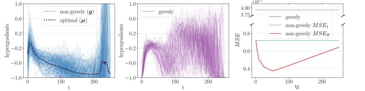Figure 1: Hypergradients on SVHN for 100 seeds in the non-greedy (left) and greedy (middle) setting. The mean squared error is also shown (right).

The first experiment tested how well hyperparameter sharing dealt with hypergradient noise and how it affected the hypergradient error, training the learning rate for LeNet on the SVHN dataset. The method did, in fact, outperform the greedy setting, significantly reducing noise for many values of $W$. Interestingly, the mean squared error of the gradient has also significantly reduced, showing the best result for $W=50$.

The effect of hyperparameter sharing on HPO

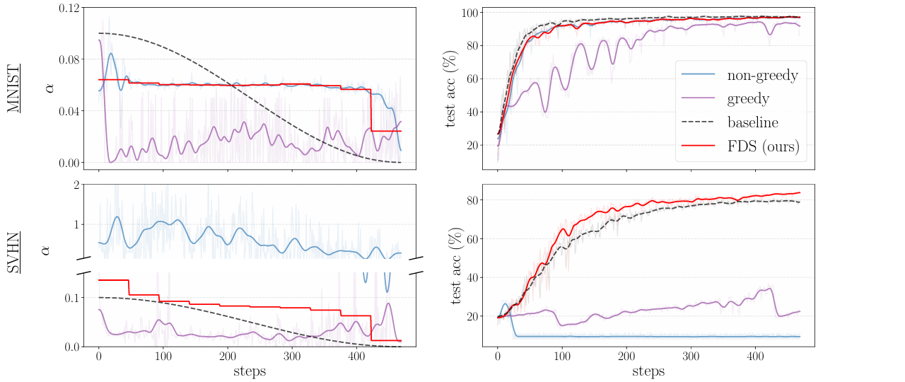Figure 2: The learning rate schedule learned on MNIST and SVHN using LeNet.

The next two experiments analyze how hyperparameter sharing affects performance of HPO on various real datasets. In the Figure 2, we can see the results of training the learning rate for LeNet on MNIST and SVHN. Despite LeNet being a relatively small architecture, making non-greedy HPO a viable option, both greedy and non-greedy HPO fail to find reasonable learning rates for training on SVHN, probably due to hypergradient variance. On the other hand, FDS stabilizes non-greedy hypergradients and allows to find learning rates that even outperform reasonable off-the-shelf schedules (cosine annealing in this case).

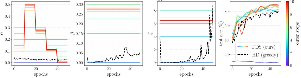Figure 3: FDS applied to SGD with momentum to learn the learning rate schedule $\alpha$, momentum $\beta$ and weight decay $\xi$.

Figure 3 shows the results of an experiment with a larger model, WideResNet-16-1, on the CIFAR-10 dataset. Due to the size of the model, non-greedy HPO without hyperparameter sharing becomes too computationally expensive, so the authors only compared FDS with a greedy method, Hypergradient Descent (HD). This experiment shows that in just 10 outer steps, FDS manages to converge to noticeably more reasonable values of the hyperparameters than HD, resulting in better test performance while still being a viable option in this setting.

FDS vs. other HPO methods

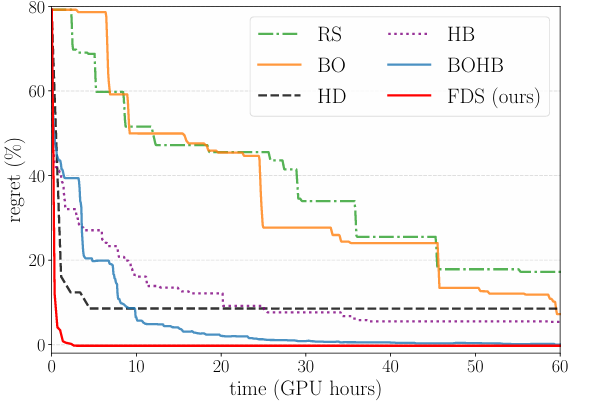Figure 4: Performance of the most popular HPO methods on CIFAR-10 for a WideResNet-16.

The last experiment aims to demonstrate why FDS is such a valuable method compared to others used before it. We can see that non-greedy methods like random search (RS), Bayesian optimization (BO), Hyperband (HB) and the combination of the latter two (BOHB), while solving for global optima, rely on trial-and-error, which makes them very slow. On the other hand, greedy methods like Hypergradient Descent (HD) are faster but solve for local optima. FDS manages to take the best of both worlds, outperforming even the next best method while converging 20 times faster.

Conclusion

FDS has been proven to be a well-balanced alternative to the state-of-the-art methods at the time, and its notable performance still makes it a strong baseline to this day. While the field of HPO has since then developed quite significantly, FDS is still worth considering in various applications, given its strengths.

Main strengths of FDS:

• Hypergradient noise reduction: hyperparameter sharing allows to combat gradient degradation, reducing the hypergradient error for optimal configurations of $W$ (for many purposes $W=50$ proved to be quite optimal).
• Accuracy: offers better accuracy without trade-offs in comparison to greedy methods.
• Convergence speed: converges much faster than trial-and-error methods.

Limitations:

• Requires differentiable hyperparameters: to use FDS with discrete hyperparameters, you will need to perform relaxation.
• Memory requirements scale linearly with the amount of hyperparameters. For example, a 12 GB GPU can train up to ~$10^3$ hyperparameters.
• Recurrent formulas are parameter-specific: each type of hyperparameter will require the derivation of its own expressions for matrices $\mathbf{A}_t$ and $\mathbf{B}_t$.