Based on the 2018 NeurIPS conference paper by Ozan Sener and Vladlen Koltun

If you find this topic interesting, please check out the original paper!

Introduction

In the realm of statistics, there is a fascinating phenomenon known as Stein’s Paradox. It states that when you need to estimate the means of three or more Gaussian random variables, you actually get a better estimate if you compute them jointly using samples from all of them, rather than estimating each one separately—even if the variables are completely independent!

This mathematical quirk serves as an early motivation for Multi-Task Learning (MTL). In modern machine learning, MTL leverages the shared inductive bias across different tasks to improve overall performance. For instance, in autonomous driving, predicting depth and segmenting pedestrians are seemingly different tasks, yet they are governed by the same physical laws of optics and scene geometry. Why learn the rules of the visual world from scratch for every single task when you can learn them once and share the knowledge?

The Problem with the Standard Approach

Typically, MTL in deep neural networks is implemented via hard parameter sharing: the network has shared parameters $\theta^{sh}$ (the feature extractor/encoder) and task-specific parameters $\theta^{t}$ (the heads/decoders).

The most common way to optimize such a model is by taking a linear combination of empirical losses:

\[\min_{\theta^{sh}, \theta^{1}, \dots, \theta^{T}} \sum_{t=1}^{T} c_t \hat{\mathcal{L}}^t(\theta^{sh}, \theta^t)\]

where $c_t$ are static or dynamically computed weights.

The flaw: This approach makes a massive assumption—that the tasks do not compete. In reality, tasks frequently conflict. Improving the loss for task A might degrade the loss for task B. When tasks compete, the linear combination forces an arbitrary trade-off, usually requiring an excruciatingly expensive grid search over the weights $c_t$ to find a “good enough” balance.

The Paradigm Shift: Multi-Objective Optimization

Instead of forcing tasks to cooperate through a weighted sum, Sener and Koltun propose casting MTL explicitly as Multi-Objective Optimization (MOO). In MOO, we accept that tasks conflict and that a single “global optimum” that minimizes all losses simultaneously simply might not exist.

Instead, the goal is to find an optimal trade-off, mathematically defined as a Pareto optimal solution.

Pareto Optimality Defined

To understand the objective, we must define two key concepts:

1. Dominance: A set of parameters $\theta$ dominates another set $\bar{\theta}$ if it is better or equal on all tasks, and strictly better on at least one task. Mathematically: $\forall t, \hat{\mathcal{L}}^t(\theta) \leq \hat{\mathcal{L}}^t(\bar{\theta})$ and $\exists i \text{ s.t. } \hat{\mathcal{L}}^i(\theta) < \hat{\mathcal{L}}^i(\bar{\theta})$.
2. Pareto Optimality: A solution $\theta^\ast$ is Pareto optimal if no other solution dominates it. The set of all such solutions forms the Pareto front.

Our new objective is to use gradient-based algorithms to smoothly navigate our model parameters until we land on this Pareto front.

The Math: MGDA and KKT Conditions

To achieve Pareto optimality, the authors turn to the Multiple Gradient Descent Algorithm (MGDA). MGDA relies on the Karush-Kuhn-Tucker (KKT) conditions for multi-objective optimization.

For a point to be Pareto stationary, two conditions must hold:

1. For task-specific parameters: $\nabla_{\theta^{t}} \hat{\mathcal{L}}^t(\theta^{sh}, \theta^t) = 0$
2. For shared parameters: there must exist weights $\alpha_1, \dots, \alpha_T \geq 0$ where $\sum_{t=1}^T \alpha_t = 1$, such that: \(\sum_{t=1}^T \alpha_t \nabla_{\theta^{sh}} \hat{\mathcal{L}}^t(\theta^{sh}, \theta^t) = 0\)

To satisfy the second condition and find a gradient direction that improves all tasks simultaneously, we must solve an optimization problem on a simplex at each training step:

\[\min_{\alpha_1, \dots, \alpha_T} \left\| \sum_{t=1}^T \alpha_t \nabla_{\theta^{sh}} \hat{\mathcal{L}}^t(\theta^{sh}, \theta^t) \right\|_2^2 \quad s.t. \sum_{t=1}^T \alpha_t = 1, \alpha_t \geq 0\]

Geometrically, this is equivalent to finding the minimum-norm point within the convex hull of the task gradients. If you think of each task as a player in a multi-directional tug-of-war over the shared weights, this algorithm calculates the exact center of force where everyone is satisfied.

The Computational Bottleneck

Here is where the elegant theory hits a brick wall of computational reality.

To solve the simplex optimization problem above, we need the gradient of each task’s loss with respect to the shared parameters: $\nabla_{\theta^{sh}} \hat{\mathcal{L}}^t$. In a deep neural network, computing this requires a separate backward pass for each task. If you have 40 tasks, you need 40 backward passes per training step. This linear scaling with the number of tasks makes standard MGDA entirely impractical for deep learning.

The Proposed Solution: MGDA-UB

To bypass this bottleneck, the authors exploit the architecture of neural networks. Let $Z = g(x; \theta^{sh})$ be the shared representations (the output of the shared encoder).

Using the chain rule, we can extract the Jacobian of the representation w.r.t the shared parameters: $\frac{\partial Z}{\partial \theta^{sh}}$. The authors prove the following upper bound:

\[\left\| \sum_{t=1}^T \alpha_t \nabla_{\theta^{sh}} \hat{\mathcal{L}}^t \right\|_2^2 \leq \left\| \frac{\partial Z}{\partial \theta^{sh}} \right\|_2^2 \left\| \sum_{t=1}^T \alpha_t \nabla_{Z} \hat{\mathcal{L}}^t \right\|_2^2\]

Notice something beautiful here? The term $\left| \frac{\partial Z}{\partial \theta^{sh}} \right|_2^2$ does not depend on $\alpha$.

This means to find the optimal $\alpha$ weights, we can drop the expensive shared-parameter gradients and optimize only using the gradients with respect to the representations $Z$:

\[\min_{\alpha} \left\| \sum_{t=1}^T \alpha_t \nabla_{Z} \hat{\mathcal{L}}^t \right\|_2^2\]

Why is this a game-changer? The gradients with respect to $Z$ ($\nabla_{Z} \hat{\mathcal{L}}^t$) can be computed for all tasks simultaneously in a single backward pass. The computational overhead of MOO effectively drops to zero.

The authors theoretically guarantee this approach with a theorem:

Theorem 1: Assuming $\frac{\partial Z}{\partial \theta^{sh}}$ is full rank, if $\alpha^{1,\dots,T}$ is the solution to the MGDA-UB problem, it will either yield a Pareto stationary point or provide a descent direction that strictly decreases all objective losses.

The Final Algorithm

The training loop elegantly comes together as follows:

1. Update task-specific parameters $\theta^t$ using their respective gradients.
2. Compute the gradients of task losses with respect to the shared representations $Z$.
3. Solve the Frank-Wolfe optimization algorithm on the simplex to find the optimal $\alpha$ weights.
4. Calculate the common descent direction $\Delta = \sum_{t=1}^T \alpha_t \nabla_{\theta^{sh}} \hat{\mathcal{L}}^t$ (effectively done via a standard backward pass weighted by $\alpha$).
5. Update shared parameters $\theta^{sh}$ using $\Delta$.

---

Experimental Results

To prove that this isn’t just theoretical wizardry, the authors evaluated MGDA-UB on three distinct benchmarks, increasing the complexity and the number of tasks.

1. MultiMNIST (Capacity Competition)

The first experiment uses MultiMNIST, where two digits are overlaid on a single image. The two tasks are classifying the top-left digit and the bottom-right digit.

Because the network has limited capacity, these two tasks heavily compete. As seen in the results, standard linear combinations (even after exhaustive grid search) fail to match the performance of training two entirely separate models (Single Task).

MGDA-UB, however, perfectly navigates the capacity competition, matching single-task performance without needing two separate networks.

Figure 1. Authors plot the obtained accuracy in detecting the left and right digits for all baselines. The grid-search results suggest that the tasks compete for model capacity. Proposed method is the only one that finds a solution that is as good as training a dedicated model for each task. Top-right is better.

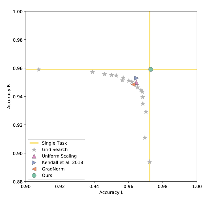
Table 1. Comparison of proposed method vs baselines on MultiMNIST.

Method	Left digit acc. $\uparrow$	Right digit acc. $\uparrow$
Single task	97.23	95.90
Uniform scaling	96.46	94.99
Kendall et al. 2018	96.47	95.29
GradNorm	96.27	94.84
Ours (MGDA-UB)	97.26	95.90

2. CelebA (Scaling to 40 Tasks)

To test scalability, the authors framed the CelebA facial attribute dataset as a 40-way multi-label classification problem. Grid search is mathematically impossible here.

Despite the massive number of tasks, MGDA-UB seamlessly scaled to 40 objectives, beating Uniform Scaling, Uncertainty Weighting (Kendall et al.), and GradNorm, achieving the lowest average error.

Figure 2. Radar charts of percentage error per attribute on CelebA. Lower is better. Authors divide attributes into two sets for legibility: easy on the left, hard on the right. Zoom in for details.

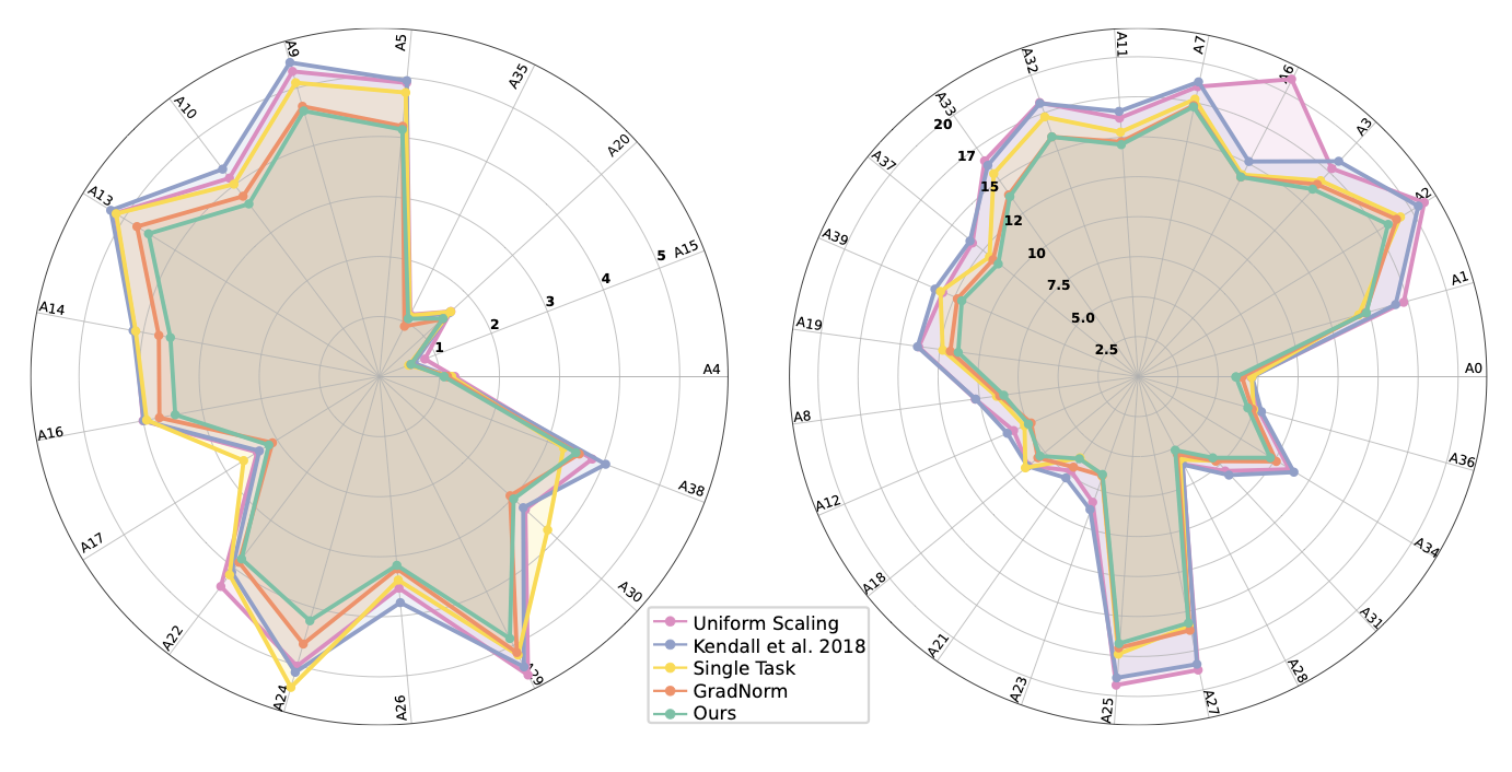
Table 2. Comparison of proposed method vs baselines on CelebA.

Method	Average error $\downarrow$
Single task	8.77
Uniform scaling	9.62
Kendall et al. 2018	9.53
GradNorm	8.44
Ours (MGDA-UB)	8.25

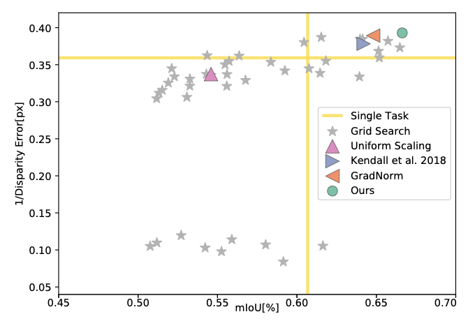
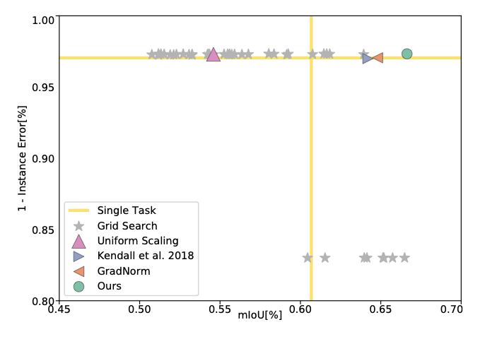
3. Cityscapes (Complex Scene Understanding)

Moving to a real-world autonomous driving analog, the model was tasked with jointly performing semantic segmentation, instance segmentation, and monocular depth estimation on the Cityscapes dataset using a ResNet-50 encoder.

Once again, MGDA-UB achieved state-of-the-art results across all three metrics. It allowed the tasks to actively cooperate, beating single-task baselines across the board.

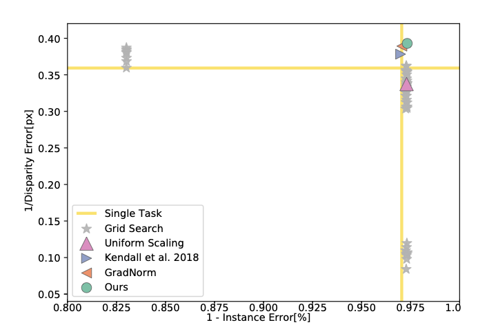
Figure 3. Authors plot the performance of all baselines for the tasks of semantic segmentation, instance segmentation, and depth estimation. They use mIoU for semantic segmentation, error of per-pixel regression (normalized to image size) for instance segmentation, and disparity error for depth estimation. To convert errors to performance measures, they use 1 - instance error and 1/disparity error. They plot 2D projections of the performance profile for each pair of tasks. Although they plot pairwise projections for visualization, each point in the plots solves all tasks. Top-right is better.

4. The Role of the Approximation (Ablation Study)

A crucial question remains: Does approximating the true MGDA with the Upper Bound (MGDA-UB) hurt performance?

The authors compared exact MGDA (multiple backward passes) against MGDA-UB. The results were startling. On CelebA (40 tasks), the training time dropped from 42.9 hours to just 1.6 hours (a ~25x speedup).

Even more surprisingly, accuracy slightly improved with the approximation. The authors hypothesize that calculating the simplex optimization in the lower-dimensional space of $Z$ (thousands of dimensions) rather than $\theta^{sh}$ (millions of dimensions) significantly reduces gradient noise, leading to higher stability.

Method	Time (h) $\downarrow$	Segm mIoU $\uparrow$	Inst err $\downarrow$	Disp err $\downarrow$	Time (h) $\downarrow$	Avg err $\downarrow$
	Scene (3 tasks)				CelebA (40 tasks)
Exact MGDA	66.1	66.13	10.28	2.59	42.9	8.33
MGDA-UB	38.6	66.63	10.25	2.54	1.6	8.25

---

Conclusion

Sener and Koltun’s paper shifts the paradigm of Multi-Task Learning from empirical weight guessing to rigorous mathematical optimization.

Key Takeaways:

1. Mathematically Sound: Formulating MTL as finding a Pareto optimum removes the need for heuristic weight tuning.
2. Highly Scalable: The MGDA-UB upper bound reduces an $O(T)$ backward pass bottleneck to a single backward pass, making gradient-based MOO practical for massive deep neural networks.
3. Theoretically Proven: Optimizing the upper bound is mathematically guaranteed to yield a Pareto stationary point (under full-rank Jacobian assumptions).
4. State-of-the-Art: It efficiently utilizes shared model capacity, achieving top performance across digit classification, multi-label prediction (up to 40 tasks), and dense computer vision tasks.