Why this paper matters
Many machine-learning problems are really problems about hidden motion. We do not directly see the true state of a system: the position and velocity of a car, the internal state of a robot, the real phase of an epidemic, or the underlying dynamics of a noisy sensor. We only see imperfect measurements. A state-space model is a standard way to describe this situation.
The paper Ensemble Kalman Filtering Meets Gaussian Process SSM for Non-Mean-Field and Online Inference asks a practical question: can we learn an unknown nonlinear dynamical system from noisy observations while also estimating the hidden states? The authors combine two ideas that are powerful in different ways:
- Gaussian processes (GPs): flexible Bayesian models for unknown functions, with uncertainty.
- Ensemble Kalman filtering (EnKF): a fast filtering method that tracks hidden states using a cloud of particles.
Their method is called EnVI: EnKF-aided Variational Inference. The online version is called OEnVI. The main message is simple: instead of training a large neural inference network to guess hidden states, use a model-based filter to do that job, and let the GP focus on learning the dynamics.
One-sentence intuition: the GP learns “how the system tends to move”, while the EnKF continuously asks “given what we just observed, where is the system now?”
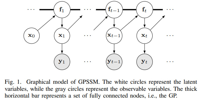
The modeling problem: hidden states and noisy observations
A state-space model has two parts. The first part says how the hidden state evolves. The second part says how observations are generated from the hidden state:
\[x_{t+1} = f(x_t) + v_t, \qquad y_t = Cx_t + e_t.\]Here $x_t$ is the hidden state, $y_t$ is the observation, $f$ is the transition function, and $v_t, e_t$ are noise terms. The matrix $C$ maps the hidden state to the observation space.
If $f$ is known and the model is linear-Gaussian, the classical Kalman filter is almost ideal. But in many realistic problems, $f$ is not known. We may only have a sequence of noisy observations and need to learn both:
- the hidden trajectory $x_0, x_1, \ldots, x_T$;
- the transition rule $f$ that generated it.
This creates a chicken-and-egg problem. To learn $f$, we need good estimates of the hidden states. To infer the hidden states, we need a good $f$.
Gaussian processes: learning a function with uncertainty
A Gaussian process is a distribution over functions. Instead of saying “the transition function must be a neural network with these weights”, a GP says: before seeing data, plausible functions are those that look smooth according to a kernel $k$.
A compact way to write this is:
\[f(\cdot) \sim \mathcal{GP}(0, k(\cdot, \cdot)).\]After seeing data, the GP gives two things at a new input:
- a mean prediction: the most likely function value;
- a variance: how uncertain the model is there.
This uncertainty is very useful in dynamical systems. If we ask the model to predict in a region it has not seen, it should not pretend to be confident. This is one reason GP state-space models, or GPSSMs, are attractive for small and medium datasets.
The difficulty is computational. A full GP becomes expensive for long time series, and in GPSSMs the inputs to the GP are hidden states, not observed data. The paper therefore uses a standard sparse-GP trick: inducing points. These are a small set of representative pseudo-inputs that summarize the transition function. Instead of carrying the whole GP over every time point, the algorithm learns a compact surrogate.
Kalman filtering and EnKF: tracking the hidden state
The Kalman filter alternates between two steps:
- Predict: use the dynamics to move the previous state estimate forward.
- Update: correct the prediction using the new observation.
In the linear-Gaussian case, this is exact. In nonlinear systems, the Ensemble Kalman Filter keeps a cloud of particles, called an ensemble, and moves each particle through the dynamics. Then it updates the whole cloud using a Kalman-style correction.
A simplified update for the mean looks like this:
\[m_t = \bar m_t + G_t(y_t - C\bar m_t),\]where $\bar m_t$ is the predicted mean, $y_t - C\bar m_t$ is the surprise in the new observation, and $G_t$ is the Kalman gain. The gain decides how much to trust the observation versus the model prediction.
For this paper, the important point is not only that EnKF is fast. It is also differentiable when implemented carefully with reparameterized noise. That means gradients can flow through the filtering procedure, so the GP parameters and variational parameters can be optimized with tools such as automatic differentiation.
How EnVI unites GPSSMs and EnKF
The paper’s central idea is to put EnKF inside variational inference for GPSSMs. Variational inference normally introduces an approximate posterior distribution $q$ and optimizes an evidence lower bound, or ELBO. In many previous GPSSM methods, the distribution over hidden states is parameterized by many extra variables or by an inference network. That can be slow, unstable, and awkward for online learning.
EnVI changes the design:
Noisy observations y_t
        |
        v
EnKF estimates hidden states x_t
        |
        v
Sparse GP learns transition f(x_t)
        |
        v
ELBO balances data fit + regularization
        |
        v
Updated model for filtering and forecasting
The approximate objective derived in the paper can be read as:
\[\mathcal L \approx \mathbb E_{q(u)}\left[\sum_{t=1}^T \log p(y_t \mid u, y_{1:t-1})\right] - \mathrm{KL}(q(x_0)\|p(x_0)) - \mathrm{KL}(q(u)\|p(u)).\]The first term rewards predictions that explain the observations. The two KL terms act as regularizers: the initial state and the GP transition should not drift too far from their priors unless the data strongly supports it.
This is a nice objective because it is interpretable. The algorithm is not just fitting observations. It is also controlling model complexity and uncertainty.
Why “non-mean-field” matters
A mean-field approximation breaks dependencies between groups of variables. This often makes optimization easier, but in a dynamical model it can be too aggressive. The hidden states and transition function are deeply linked: changing the transition function changes the plausible hidden trajectory, and changing the hidden trajectory changes what transition function is learned.
EnVI keeps this relationship more naturally. The EnKF state estimates depend on the GP transition, and the GP is learned from those filtered states. This is why the paper calls the method non-mean-field: it does not pretend that the latent states and GP dynamics are independent.
Online learning: OEnVI
The online version, OEnVI, processes data one time step at a time. At each new observation it performs the same basic cycle:
- sample or use the current GP surrogate;
- predict the ensemble forward;
- update the ensemble with the new observation;
- update model and variational parameters using the local objective.
The online objective has the same spirit as the offline one:
\[\mathcal L_t = \mathbb E_{q(u)}[\log p(y_t \mid u, y_{1:t-1})] - \mathrm{KL}(q(u)\|p(u)).\]This matters because many systems do not arrive as a fixed dataset. Sensors, robots, vehicles, and monitoring systems stream data continuously. A method that requires the entire sequence at training time is less convenient there. OEnVI is designed to update as data arrives.
What tasks does this combination solve?
The GP-EnKF combination is useful for several related tasks:
| Task | What the model does | Why the combination helps |
|---|---|---|
| Filtering | Estimate current hidden state from noisy observations | EnKF corrects predictions using new measurements |
| Dynamics learning | Learn the unknown nonlinear transition function | GP models flexible dynamics and reports uncertainty |
| Forecasting | Predict future observations and uncertainty | The learned GP transition can be rolled forward |
| Online inference | Update the model as data streams in | OEnVI avoids a heavy inference network trained on full sequences |
The key design choice is that EnKF handles the state-estimation part, while the GP handles the unknown-function part. Variational inference ties them together with a principled training objective.
Experimental results: what was most impressive?
The authors test the methods on synthetic and real datasets. The exact numbers are less important than the pattern: EnVI is usually more accurate, more robust, or faster to train than competing GPSSM and neural state-space methods.
1. Linear-Gaussian tracking: close to the Kalman filter
The authors first use a setting where the classical Kalman filter is available as a strong reference: a linear-Gaussian car-tracking model. EnVI and OEnVI do not receive the true physical transition model, only noisy observations.
Even so, their state estimates are close to the Kalman filter baseline. The reported latent-state RMSE values are:
- Kalman filter: 0.5252;
- EnVI: 0.6841;
- OEnVI: 0.7784;
- raw observations versus latent states: 0.9872.
This experiment is a sanity check. If a learned GPSSM cannot do well on a linear-Gaussian system, it is hard to trust it on nonlinear ones. EnVI passes this check convincingly. OEnVI is less accurate at the beginning because it learns sequentially, but the paper reports that after more online data it improves substantially.
2. Kink function: learning nonlinear dynamics under noise
The kink function is a classic GPSSM test. It is a one-dimensional nonlinear transition that is simple enough to visualize but hard enough to expose bad uncertainty estimates.
Across three observation-noise levels, EnVI obtains the best transition-function fit among the compared methods. For example, at the lowest noise level, EnVI reports MSE 0.0046, while AD-EnKF reports 0.0285, VCDT 0.2057, and vGPSSM 1.0410. At high noise, EnVI still performs best: MSE 0.5315, compared with 1.3489 for AD-EnKF, 1.4035 for VCDT, and 1.9584 for vGPSSM.
The visual result is also important: EnVI learns both the shape of the kink and a reasonable uncertainty band. The paper argues that AD-EnKF can become overconfident because it uses a deterministic neural transition model, while EnVI keeps uncertainty through the GP.
Another striking result is convergence. On the kink experiment, EnVI reaches good performance after roughly 300 iterations, whereas vGPSSM and VCDT require many more iterations and more runtime. This supports the authors’ claim that removing a large inference network makes optimization easier.
3. Real time-series forecasting: strong small-data performance
The paper also evaluates five public system-identification datasets: Actuator, Ball Beam, Drive, Dryer, and Gas Furnace. The model trains on the first half of each sequence and forecasts the second half. The reported metric is 50-step-ahead RMSE.
EnVI is best on four of the five datasets and competitive on the fifth. Its RMSEs are:
- Actuator: 0.657;
- Ball Beam: 0.055;
- Drive: 0.703;
- Dryer: 0.125;
- Gas Furnace: 1.388.
The Drive dataset is the main exception: PRSSM reports 0.647, better than EnVI’s 0.703. But overall, the results are strong, especially because these datasets are relatively small. That is exactly the regime where GP-based models can be attractive compared with large neural models.
4. Online NASCAR dynamics: OEnVI wins clearly
For online learning, the authors use a NASCAR-shaped latent trajectory and compare OEnVI with SVMC and VJF. The prediction RMSEs are:
- OEnVI: 1.8780;
- SVMC: 4.6682;
- VJF: 10.8499.
This is one of the clearest experimental wins in the paper. OEnVI tracks and predicts the latent trajectory much better than the alternatives. The authors attribute this to the EnKF-based approximation of the latent-state distribution: it is structured enough to be stable, but flexible enough to work online.
Takeaways and limitations
The paper is interesting because it does not simply replace everything with a neural network. It combines a probabilistic non-parametric model with a classical filtering algorithm, then trains the whole system with variational inference.
The main takeaways are:
- GPSSMs are useful when the transition dynamics are unknown and nonlinear.
- EnKF provides a practical way to infer hidden states without a heavy inference network.
- The resulting ELBO has a clear interpretation: fit the observations, but regularize the initial state and transition function.
- OEnVI makes the method suitable for streaming data.
- The strongest empirical results are on nonlinear dynamics learning and online tracking.
There are also natural limitations. EnKF relies on Gaussian-style updates, so it may struggle in strongly non-Gaussian settings where particle filters are more appropriate. The paper mainly uses a linear emission model, although EnKF can be extended to nonlinear emissions. Finally, the conclusion notes that time-varying dynamical systems remain an important direction for future work.
Useful links for readers
- Original paper on arXiv: Ensemble Kalman Filtering Meets Gaussian Process SSM
- Authors’ GPSSM code repository: zhidilin/gpssmProj
- A classic free book on Gaussian processes: Gaussian Processes for Machine Learning
- Intuitive Kalman filtering book with Python code: Kalman and Bayesian Filters in Python
- Practical GP library documentation: GPyTorch variational and approximate GPs