Based on the state-space regression framework for Student-t processes.
This post explains how to turn a standard Gaussian-process-style regression problem into a robust, scalable state-space model. The core idea is simple: keep the analytical structure of Gaussian-process inference, but replace the fixed Gaussian uncertainty with a Student-t process so that the model becomes much more tolerant to outliers.
Introduction
Gaussian processes (GPs) are one of the most elegant tools for non-parametric regression. They provide closed-form posterior predictions, uncertainty estimates, and a principled way to encode prior structure through kernels. But in practice, standard GP regression has two major weaknesses:
- Computational cost: the naive implementation requires matrix inversion and scales as $O(n^3)$.
- Sensitivity to outliers: the posterior variance depends only on input locations, not on observed values, so a single bad observation does not automatically increase uncertainty.
For many real-world time series, these limitations are a problem. Sensor failures, missing values, and occasional large spikes are common, and a model should react to them instead of treating every observation as equally trustworthy.
The method discussed here replaces the Gaussian assumption with a Student-t process (TP) and then exploits a state-space representation to make inference efficient. The result is a model that is both robust and fast.
Gaussian processes in one page
A Gaussian process is a distribution over functions:
\[f(x) \sim \mathcal{GP}(\mu(x), k(x,x'))\]which means that for any finite set of inputs $x_1,\dots,x_n$, the vector of function values is jointly Gaussian:
\[(f(x_1), \ldots, f(x_n))^T \sim \mathcal{N}(\boldsymbol{\mu}, K), \qquad K_{ij} = k(x_i, x_j).\]For GP regression, the posterior mean and variance at a test point $x_*$ are
\[\mathbb{E}[f(x_*)] = k_*^T K^{-1} y,\] \[\mathbb{V}[f(x_*)] = k(x_*,x_*) - k_*^T K^{-1} k_*.\]The problem is visible in the variance formula: the uncertainty depends only on the kernel geometry and the training inputs, not on the actual observed values $y$. If the data contains a strong outlier, the model does not automatically become more uncertain about that region.
Why Student-t processes help
The Student-t distribution has heavier tails than the Gaussian, which makes it much more forgiving to unexpected observations. For a vector $y \in \mathbb{R}^n$,
\[y \sim \mathrm{MVT}(\mu, K, \nu)\]with density
\[p(y|\mu,K,\nu) = \frac{\Gamma\!\left(\frac{\nu+n}{2}\right)} {\Gamma\!\left(\frac{\nu}{2}\right)\left((\nu-2)\pi\right)^{n/2}|K|^{1/2}} \left( 1 + \frac{(y-\mu)^T K^{-1}(y-\mu)}{\nu-2} \right)^{-\frac{\nu+n}{2}}.\]As $\nu \to \infty$, this distribution approaches a Gaussian.
A useful way to think about the Student-t distribution is as a scale mixture of Gaussians:
\[\gamma \sim \mathrm{IG}\!\left(\tfrac{\nu}{2}, \tfrac{\nu-2}{2}\right), \qquad y \mid \gamma \sim \mathcal{N}(\mu, \gamma K) \quad \Longrightarrow \quad y \sim \mathrm{MVT}(\mu, K, \nu).\]So the Student-t is still Gaussian at its core, but with a random scale factor $\gamma$. That single random variable is what makes the model adaptive: unusual observations can be explained by a larger local scale, which effectively reduces their influence.
Student-t process regression
A Student-t process is the function-space analogue of the multivariate Student-t distribution:
\[f(x) \sim \mathrm{TP}(\mu(x), k(x,x'), \nu)\]if every finite collection of function values follows a multivariate Student-t law.
For regression, the crucial point is that the conditional distribution of one block of variables given another retains the same structure. If the joint vector is Student-t distributed, then the conditional posterior is also Student-t, with a mean similar to the GP case but with a variance scaling term that depends on the observations.
For a test point $x_*$, the predictive distribution can be written as
\[f(x_*) \mid D \sim \mathrm{MVT}\!\left( k_*^T K^{-1} y,\; \frac{\nu - 2 + \beta}{\nu - 2 + n} \bigl(k(x_*,x_*) - k_*^T K^{-1}k_*\bigr),\; \nu + n \right),\]where
\[\beta = y^T K^{-1}y.\]This is the most important difference from GP regression:
- in a GP, uncertainty is fixed by the kernel and the input geometry;
- in a TP, uncertainty grows when the data looks suspicious.
That makes the posterior variance much more informative in the presence of outliers.
The training objective
Hyperparameters are learned by maximizing the marginal likelihood, or equivalently minimizing the negative log marginal likelihood. For the TP model, the objective takes the form
\[\mathcal{L}(\theta) = \frac{n}{2}\log\!\bigl((\nu-2)\pi\bigr) + \frac{1}{2}\log|K| - \log\Gamma\!\left(\frac{\nu+n}{2}\right) + \log\Gamma\!\left(\frac{\nu}{2}\right) + \frac{\nu+n}{2}\log\!\left(1+\frac{\beta}{\nu-2}\right),\]where $\beta = (y-\mu)^T K^{-1}(y-\mu)$.
The learned parameters are:
- $\theta$: kernel hyperparameters,
- $\sigma_n^2$: noise level,
- $\nu$: degrees of freedom, which control tail heaviness.
Smaller $\nu$ means heavier tails and stronger robustness.
From Gaussian processes to state-space models
The key trick behind the efficient algorithm is that many one-dimensional temporal kernels admit a state-space representation. In that form, the GP is no longer computed by manipulating the full covariance matrix directly. Instead, it is represented as a linear dynamical system, and inference can be carried out with Kalman filtering.
A temporal GP
\[f(t) \sim \mathrm{GP}(0, k(t,t'))\]can be rewritten as a continuous-time stochastic differential equation (SDE):
\[d\mathbf{f}(t) = F\mathbf{f}(t)\,dt + L\,dW(t),\]with observations
\[y(t_k) = H\mathbf{f}(t_k) + \varepsilon_k.\]In discrete time, this becomes
\[\mathbf{f}_k = A_{k-1}\mathbf{f}_{k-1} + \mathbf{q}_{k-1}, \qquad \mathbf{q}_{k-1} \sim \mathcal{N}(0, Q_{k-1}),\] \[y_k = H\mathbf{f}_k + \varepsilon_k.\]This transformation is the reason the method becomes scalable: rather than working with all pairwise correlations at once, we propagate a compact latent state forward in time.
The Student-t process as a state-space model
The same idea extends to the Student-t process by introducing a random scaling variable $\gamma$. The state-space model becomes a Gaussian SDE with a shared scale:
\[\mathbf{f}(0) \sim \mathcal{N}(0, \gamma P_0),\] \[d\mathbf{f}(t) = F\mathbf{f}(t)\,dt + L\,dW(t), \qquad W(t) \sim \mathcal{N}(0, \gamma Q_c),\] \[y(t_k) = H\mathbf{f}(t_k) + \varepsilon_k.\]In discrete time, the same scaling appears in the process covariance:
\[\mathbf{f}_0 \sim \mathcal{N}(0, \gamma P_0), \qquad \mathbf{q}_{k-1} \sim \mathcal{N}(0, \gamma Q_{k-1}).\]This gives the model the heavy-tailed behavior of the Student-t process while preserving the linear-Gaussian structure needed for Kalman-style inference.
Filtering: the forward pass
Inference is carried out by a forward recursion that is closely analogous to the Kalman filter.
At each step, the algorithm maintains a current estimate of the latent state together with its uncertainty, plus two Student-t-specific variables that control how strongly the next observation should affect the posterior.
The recursion has four conceptual stages:
Prediction
The model first propagates the previous estimate forward in time using the state-space dynamics.
Innovation
It then compares the prediction with the new observation and measures how surprising that observation is.
Scale update
This is the key Student-t feature. If the innovation is unusually large, the model increases its scale variable, which inflates uncertainty and reduces the influence of that suspicious observation.
State update
Finally, the latent state estimate is corrected using the innovation, but now with the outlier-robust weighting produced by the scale update.
So the forward pass behaves like a Kalman filter, but with an adaptive mechanism that automatically softens the impact of outliers instead of treating every observation equally.
Smoothing: the backward pass
Filtering gives good online estimates, but if the full sequence is available, the posterior can be improved with a backward smoothing pass.
This second pass propagates information in reverse time and refines each latent state using both the past and the future.
The result is a globally consistent trajectory estimate with the same robustness benefits as the forward pass. In practice, smoothing usually produces a cleaner reconstruction than filtering alone, especially when the observations contain noise spikes or corrupted segments.
Marginal likelihood and learning
The model parameters are learned by iterating the filtering procedure and minimizing the negative log marginal likelihood. In the state-space form, the objective accumulates contributions from each step:
\[\mathcal{L}(\theta) = \sum_{k=1}^{n} \left[ \frac{1}{2}\log\bigl((\nu-2)\pi\bigr) + \frac{1}{2}\log|S_k(\theta)| + \log\Gamma\!\left(\frac{\nu_{k-1}}{2}\right) - \log\Gamma\!\left(\frac{\nu_k}{2}\right) + \frac{\nu_k}{2} \log\!\left( 1 + \frac{v_k(\theta)^T S_k(\theta)^{-1} v_k(\theta)}{\nu_{k-1}-2} \right) \right].\]The payoff is computational: if the latent state dimension is $m \ll n$, the cost becomes approximately
\[O(nm^3) \approx O(n),\]instead of $O(n^3)$ for the naive covariance-matrix approach.
Experiments
The experiments in the presentation compare naive inference with the state-space implementation on both synthetic and real-world data.
Experiment 1: computational efficiency
The first experiment demonstrates the speed advantage of the state-space formulation. Instead of building and factorizing the full covariance matrix, the model updates a compact latent state sequentially. This is where the linear-time scaling becomes visible in practice.
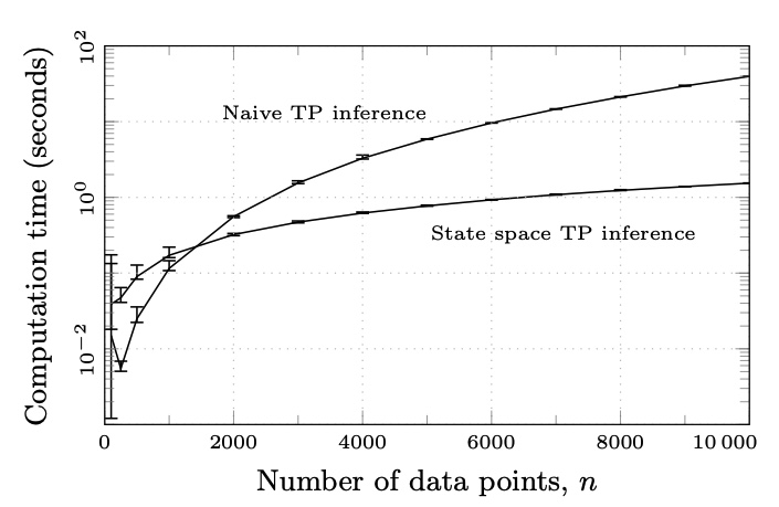
Figure 1: computational efficiency of naive inference versus the state-space method.
Experiment 2: robustness on synthetic and real data
The second experiment compares several data regimes:
- Synth A: Gaussian noise,
- Synth B: Student-t noise,
- Synth C: a mixture with outliers,
- Electricity: hourly household electricity consumption,
- Stock (Apple): log-prices over a long time span.
These settings test both accuracy and robustness. On clean Gaussian data, the GP and TP behave similarly. On contaminated data, the Student-t model is more stable and produces more meaningful uncertainty estimates.
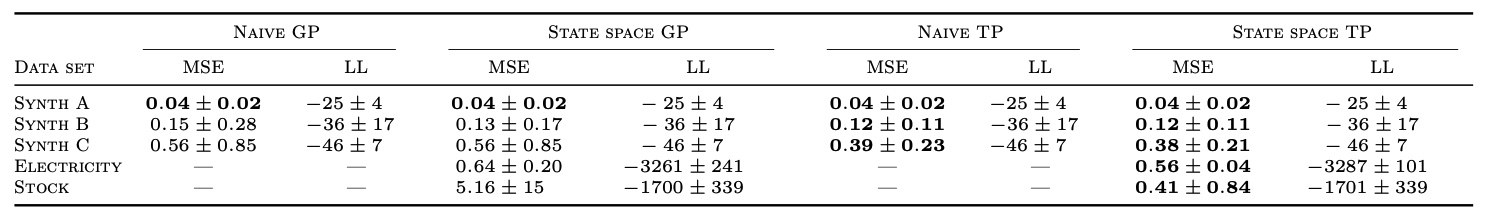
Figure 2: comparison of naive and state-space inference for GP and TP, with average MSE and log-likelihood.
Experiment 3: missing data interpolation
A particularly useful application is interpolation of missing or unreliable measurements. In such settings, the Student-t process is usually more conservative around suspicious regions and more confident elsewhere, which improves reconstruction quality.
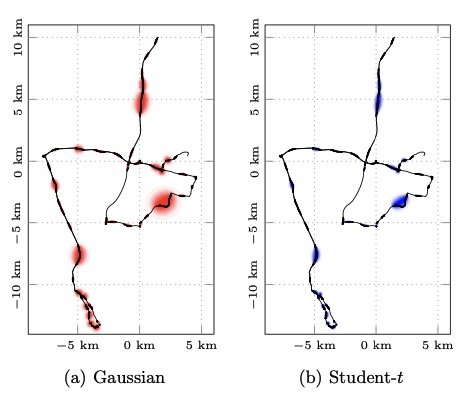
Figure 3: interpolation of missing observations with wider uncertainty around corrupted regions.
Conclusion
Student-t process regression gives a simple but powerful upgrade over standard Gaussian-process regression:
- it keeps the Bayesian, analytical nature of GP inference;
- it reacts to outliers through adaptive uncertainty;
- and, with a state-space representation, it becomes scalable enough for long time series and online inference.
The main message is that robustness and efficiency do not have to be in conflict. By combining heavy-tailed probabilistic modeling with Kalman-style inference, we get a method that is practical for real data and still mathematically elegant.
Main takeaways
- GPs are elegant but brittle when the data contains outliers.
- Student-t processes add robustness through heavy tails and observation-dependent uncertainty.
- State-space inference makes the method scalable, turning $O(n^3)$ inference into an approximately linear-time algorithm for temporal kernels.
- Filtering and smoothing remain analytical, so the model stays interpretable and easy to optimize.